Exact Reparameterization of B-Spline Mixtures for Variational Inference
Implicit gradients, low-variance sampling, and the limits of automatic smoothing
Overview. This post studies exact sampling and reparameterization for variational distributions constructed from normalized B-spline mixtures. The main observation is that the mixture CDF is a degree-raised B-spline whose coefficients are cumulative sums of the mixture weights. This gives an exact inverse-CDF sampler and implicit pathwise gradients without a Concrete relaxation or an inner Markov chain. In numerical experiments, randomized stratification reduced gradient variance by approximately 84 times compared with independent sampling at equal inverse-CDF cost. I also examine why the ELBO Hessian is not generally a measure of estimator precision, and how penalty scaling distinguishes variance-based smoothing from population model correction.
One of the recurring difficulties in variational inference is that making an approximate posterior more expressive usually makes it harder to sample from and differentiate through. Gaussian variational families are convenient largely because they admit a simple reparameterization: we sample a standard normal variable and transform it using parameters supplied by the encoder. Once we move beyond Gaussians, finding an equally convenient representation becomes more difficult.
I was looking at a variational family constructed from mixtures of normalized B-spline densities, introduced in the spline-based variational inference work of Shao, Yu and Feng (2024). The appeal of this family is fairly clear. B-splines are locally supported, their shape can be controlled through mixture weights, and evaluating the resulting density is inexpensive. The less convenient part is sampling. The original approach uses Metropolis–Hastings together with a Concrete relaxation, which makes differentiation possible but also introduces additional computation and a discrepancy between the distribution being optimized and the distribution actually sampled.
It turns out that this difficulty can be avoided without changing the variational family. The main observation is that the CDF of a normalized B-spline mixture has an especially simple representation: it is another B-spline, one degree higher, whose coefficients are cumulative sums of the original mixture weights. This allows us to sample by CDF inversion and obtain pathwise derivatives through implicit differentiation. The resulting sampler also makes randomized stratification particularly effective; in the numerical experiment considered here, using 32 stratified samples reduced gradient variance by a factor of about 84 compared with independent sampling at the same inverse-CDF cost.
While studying this construction, I also looked at the question of automatically selecting a roughness penalty for the spline weights. That led to a somewhat different issue. Although the ELBO is concave in the mixture weights, its Hessian is entirely determined by the entropy of the variational distribution. The target distribution contributes no curvature. As a consequence, directly using this Hessian in a smoothing-parameter update can lead to pathological behaviour, and more generally, it is important to distinguish regularization that reduces estimation variance from regularization that changes the population optimum.
I’ll develop these two parts in turn, beginning with the sampling problem.
Key mathematical results
The analysis establishes several useful properties of spline variational families.
Exact inverse-CDF sampling. For a normalized B-spline mixture \(q_\gamma(e)=\sum_k\gamma_k b_k(e)\), the CDF is a degree-raised B-spline with cumulative-sum coefficients:
This provides exact sampling through \(e=F_\gamma^{-1}(u)\), where \(u\sim U(0,1)\).
Implicit reparameterization gradients. Differentiating the inverse-CDF equation gives
This avoids differentiating through the numerical root solver and provides pathwise gradients without a Concrete relaxation.
The geometry of the ELBO. For fixed support and basis functions, the ELBO Hessian in mixture-weight coordinates satisfies
The target-density contribution is linear in the weights, so this curvature comes entirely from entropy. It should not automatically be interpreted as estimator precision.
Variance smoothing versus population correction. In the exact \(T=2\) IWAE experiment, the RISE-optimal penalty grows approximately as \(\lambda_n^*\approx 0.17n\). Its effect therefore persists on the population-objective scale, rather than vanishing with estimation uncertainty.
The spline mixture
Consider a collection of B-spline basis functions \(B_{k,\rho}\) of degree \(\rho\), defined on a clamped knot sequence over \([0,1]\). A standard B-spline basis function is nonnegative but does not generally integrate to one. We can turn each basis function into a probability density by normalizing it:
Given weights \(\gamma=(\gamma_1,\ldots,\gamma_K)\) on the probability simplex, define
This is a density because each \(b_k\) integrates to one and the mixture weights sum to one. Increasing a particular weight puts more mass in the region supported by its corresponding basis function, while the overlap between neighbouring B-splines allows the overall density to vary smoothly.
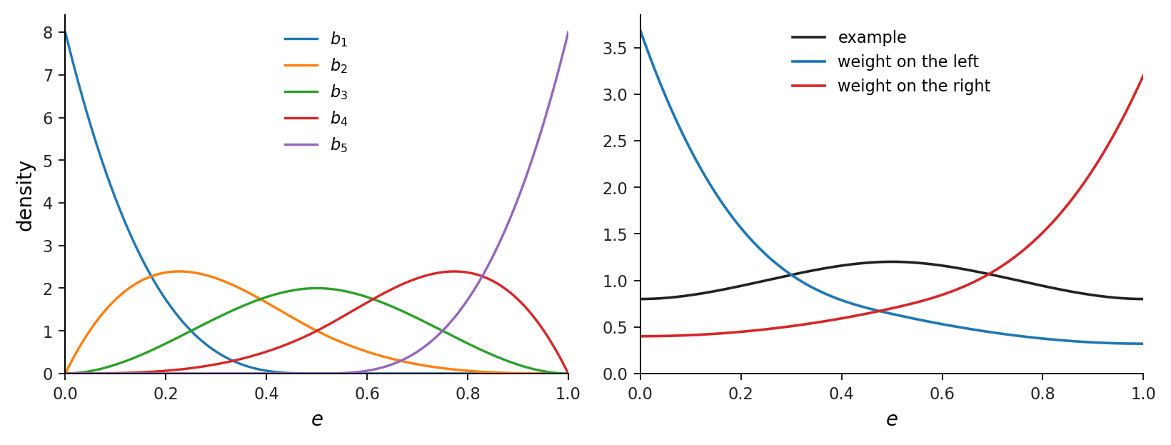
In variational inference we can use a neural network to predict these weights, together with location and scale parameters. For a latent variable \(z\), the construction takes the form
For several latent coordinates, we can use a separate spline mixture for each coordinate, giving a mean-field family. The mixture weights are conveniently parameterized through logits, \(\gamma=\operatorname{softmax}(\eta)\), so positivity and normalization are automatic.
Sampling from such a mixture is easy if differentiability is not a concern. We first draw an index \(C\) from a categorical distribution with probabilities \(\gamma\), then sample from \(b_C\). This produces exactly the required distribution, but the discrete component choice is not directly differentiable with respect to the weights.
The Concrete relaxation provides a way around this by replacing the categorical selection with a differentiable vector of approximately one-hot weights. If \(w_k\sim b_k\) independently, the relaxed sample is
where \(u(\Lambda)\) is a Concrete random vector and \(\Lambda\) is its temperature. As the temperature approaches zero, the relaxation approaches a categorical choice. At any positive temperature, however, the sample is a convex combination of draws from several components rather than a draw from one selected component.
That changes the distribution in a systematic way. For example, if \(m_k=\mathbb E[w_k]\), an expansion around zero temperature gives
The first-order change in the mean is zero, but the first-order change in variance is nonpositive. In a numerical check using one million draws with common random numbers, the observed slope of the second moment was \(-0.10672\), compared with the theoretical value \(-0.10775\). The relative difference was approximately \(0.96\%\).
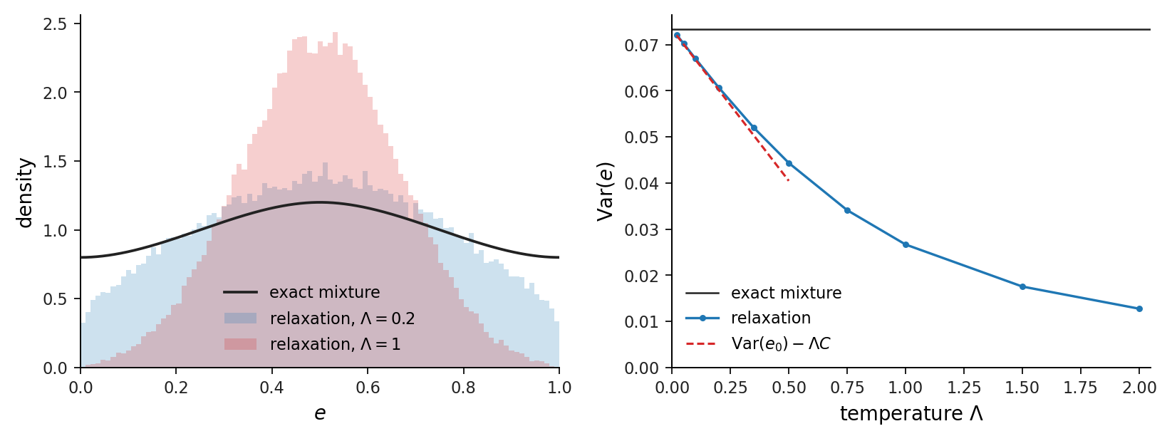
This does not mean that continuous relaxations are inherently unsuitable. They can be quite useful when an exact reparameterization is unavailable. But here the underlying distribution has enough structure that the relaxation turns out to be unnecessary.
The CDF of a Normalized B-Spline Mixture
The key fact comes from the antiderivative formula for B-splines.
If we integrate a degree-\(\rho\) B-spline expansion, the result can be represented as a degree-\((\rho+1)\) spline on an appropriately extended knot sequence. Its new coefficients are cumulative sums of the original coefficients multiplied by their corresponding basis integrals.
For the normalized mixture, those integrals cancel with the normalizing constants. If we write
and define
then
Here \(\bar B_{m,\rho+1}\) denotes the degree-raised B-spline basis with one additional repeated boundary knot at each end.
The point is that we do not need to integrate the basis numerically. We only need to take the cumulative sum of the mixture weights and evaluate a spline of degree one higher. For example, if the mixture weights are
then the CDF coefficients are simply
The final coefficient is one because the mixture weights sum to one. If all weights are positive, the density is positive throughout the interior of its support, and the CDF is strictly increasing there.
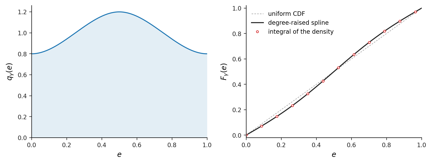
This gives an immediate sampling procedure. Draw \(u\sim U(0,1)\) and solve
The solution \(e=F_\gamma^{-1}(u)\) has exactly the desired mixture distribution, apart from the numerical tolerance used to solve the equation. In particular, we no longer need to draw a categorical component or introduce any relaxation.
The inverse can be computed efficiently because the CDF is polynomial within each knot span. We first locate the relevant span using the CDF values at the knots, initialize the root using linear interpolation, and apply Newton’s method with a bisection safeguard. Only \(\rho+1\) basis functions are nonzero locally, so evaluating the polynomial at each iteration does not require traversing the full spline basis.
There is still the question of differentiation. We could, in principle, backpropagate through every iteration of the root solver, but doing so is unnecessary.
Technical note Why the CDF of a B-spline mixture has cumulative-sum coefficients Degree elevation turns the mixture CDF into a higher-degree spline. The normalization constants cancel, so the coefficients are cumulative sums of the mixture weights and the integral does not have to be computed numerically.
Consider a B-spline basis of degree \(\rho\) on a clamped knot vector
We normalize each basis function \(B_{k,\rho}\) to obtain a probability density:
For weights \(\gamma\) on the probability simplex, the mixture is
The objective is to represent
as another spline, without performing numerical integration.
The derivative identity
A standard B-spline derivative identity is
with indices interpreted on the degree-raised, boundary-extended knot vector.
Suppose we express the CDF as
Differentiating the expansion and collecting the coefficients of the degree-\(\rho\) basis gives
But the derivative of the CDF must equal the original density:
Matching coefficients therefore gives
Since \(F_\gamma(0)=0\), the initial coefficient is \(c_0=0\), and hence
Thus
with the coefficient at \(m=0\) equal to zero.
The final coefficient is
which also ensures \(F_\gamma(1)=1\).
The cancellation of the normalization constants \(a_k\) is the crucial feature. For an ordinary spline expansion, antiderivative coefficients require knot-dependent scaling. For a mixture of normalized B-splines, the coefficients are simply cumulative probabilities.
This is what makes inverse-CDF sampling especially convenient for this family.
Implicit Reparameterization Gradients for B-Spline Mixtures
The inverse sample is defined implicitly by
Keeping \(u\) fixed and differentiating with respect to the mixture weight \(\gamma_k\) gives
Since
and
we obtain
The derivatives with respect to the unconstrained logits then follow by applying the softmax Jacobian. This is an instance of implicit reparameterization, as developed by Figurnov, Mohamed and Mnih (2018), but the spline representation means that both the CDF and its parameter derivative can be evaluated without numerical integration.
In the implementation, the root search is performed without tracking its iterations through automatic differentiation. Once a sufficiently accurate root \(e_0\) has been obtained, we make one differentiable Newton correction,
where the denominator is detached from the computational graph. The numerical value changes only by the remaining root error, while the backward pass uses the required implicit derivative.
Under standard differentiability and domination assumptions, expectations can be written as
and differentiation can be moved inside the expectation. The resulting pathwise gradient is therefore unbiased.
In the numerical checks, the maximum CDF round-trip error in double precision was \(7.8\times10^{-16}\), and the implicit gradient agreed with finite differences to \(7.3\times10^{-11}\). A probability-integral-transform check with 200,000 samples gave a Kolmogorov–Smirnov \(p\)-value of \(0.985\). Across 10,000 independent gradient experiments, no component rejected zero bias after Bonferroni correction.
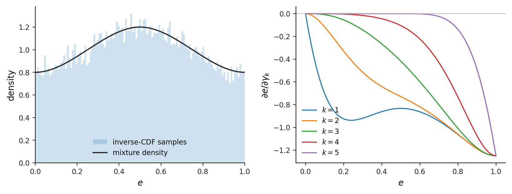
The theoretical result is exact for the stated mixture family; the numerical tests establish that the implemented inversion and differentiation are accurate to the reported tolerances.
Technical note Implicit reparameterization gradients: a worked example with B-splines The pathwise gradient follows by differentiating the inverse-CDF equation at fixed randomness. The note records the softmax chain rule, a two-component closed form, the detached Newton correction, and the finite-difference check.
Sampling from a distribution is straightforward once its inverse CDF is available. The more interesting question for variational inference is how to differentiate a sample with respect to the parameters of the distribution.
Let
Rather than treating inverse-CDF sampling as an algorithm, we can treat it as the solution of the equation
This allows us to apply implicit differentiation.
Differentiating with respect to mixture weights
At fixed \(u\), differentiation with respect to \(\gamma_k\) yields
We know that
and, from the linear mixture representation,
Thus the implicit derivative is
This is the ambient-coordinate derivative. In practice, the weights satisfy the simplex constraint and are parameterized by logits \(\eta\).
With
the softmax Jacobian is
Applying the chain rule gives
This form is useful because the derivative automatically respects the simplex constraint and is invariant to adding the same constant to every logit.
A simple two-component example
To see the calculation explicitly, take two normalized degree-zero B-spline densities:
If the mixture weights are \((\gamma,1-\gamma)\), then
Its CDF is
Therefore the inverse is available explicitly:
On the first branch, differentiating directly gives
This agrees with implicit differentiation because, along the simplex, the derivative of the CDF with respect to \(\gamma\) on this branch is \(2e\), while \(q_\gamma(e)=2\gamma\).
The same calculation can be performed on the second branch. The derivative is well defined away from the branch boundary \(u=\gamma\), which occurs with probability zero for a continuous uniform draw.
Implementing the gradient
For higher-degree splines, the inverse generally does not have a convenient closed-form expression, but the implicit derivative remains available.
The implementation proceeds by solving \(F_\gamma(e)=u\) using safeguarded Newton iteration. Once an accurate numerical solution \(e_0\) has been obtained, one differentiable correction can install the appropriate backward derivative:
The root \(e_0\) is treated as a constant during this correction. The denominator is also detached; otherwise differentiating through it introduces terms associated with the Newton update rather than simply the implicit derivative at the root.
Checking the derivative numerically
A direct implementation check uses central finite differences in the logit coordinates:
where \(e_j\) is the \(j\)-th coordinate vector.
The finite-difference derivative can then be compared with the analytic implicit derivative
The comparison should use the same base uniform \(u\) for both perturbed parameter values, since the derivative is defined at fixed randomness. Values of \(u\) extremely close to a knot boundary can be avoided in an initial diagnostic because finite-difference perturbations may change the polynomial branch being evaluated.
In the numerical evaluation reported here, the implicit gradient and finite differences agreed to \(7.3\times 10^{-11}\). The double-precision CDF round-trip error was below \(7.8\times 10^{-16}\).
These checks support the numerical implementation of a derivative that follows analytically from the implicit-function equation.
Variance Reduction with Randomized Stratification
Having a differentiable inverse-CDF sampler is useful on its own, but it also changes how we can approach Monte Carlo variance reduction. Instead of working with a discrete mixture indicator and separate component draws, the entire randomness of a one-dimensional sample is represented by a single uniform variable.
Suppose we want to estimate a gradient using \(S\) samples. Ordinary Monte Carlo draws \(u_1,\ldots,u_S\) independently from \(U(0,1)\). A perfectly valid outcome is that several samples fall into one narrow region of the interval while another region receives none. The estimator is still unbiased, but this uneven coverage can contribute substantially to its variance.
Randomized stratification avoids that particular source of randomness. Divide \([0,1]\) into \(S\) equal intervals and draw one uniform point from each:
Each point is random within its assigned interval. Averaging the transformed gradient evaluations remains unbiased, since the strata partition the integration domain with equal weights.
The reason this works well with inverse-CDF sampling is that the transformation is monotone. Covering the uniform interval evenly means that we also cover the quantile range of the spline distribution evenly. For sufficiently regular gradient integrands, this can remove a large amount of sampling variability.
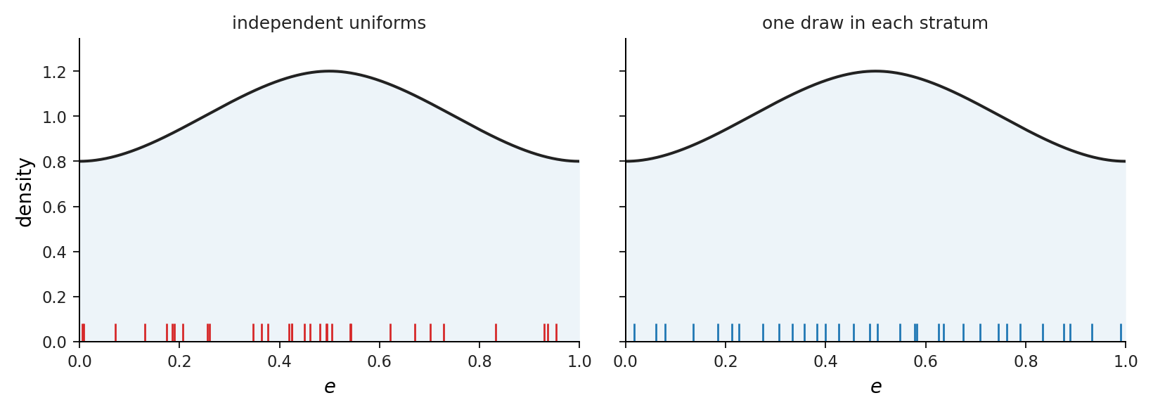
I compared independent sampling, antithetic sampling, randomized stratification, and scrambled Sobol sampling using 32 inverse-CDF evaluations per gradient estimate. The measured mean gradient variances were:
Mean gradient variance at 32 inverse-CDF evaluations. Each entry is the mean ± the jackknife standard error over eight randomizations.
| Sampling design | Mean gradient variance |
|---|---|
| Independent | (8.40 ± 2.70) × 10−4 |
| Antithetic | (1.07 ± 0.45) × 10−3 |
| Randomized strata | (1.00 ± 0.35) × 10−5 |
| Scrambled Sobol | (2.26 ± 1.33) × 10−5 |
Randomized stratification gave an approximately 84-fold reduction in variance relative to independent sampling, while scrambled Sobol gave an approximately 37-fold reduction. Antithetic sampling was actually worse for this particular integrand. These results used eight independent randomizations for each design, so the exact ratios should be understood as empirical comparisons rather than general guarantees.
The advantage remained substantial in a larger randomization experiment. With 64 draws and 256 independent randomizations, the trace of the gradient covariance relative to independent sampling was \(0.00302\) for randomized stratification and \(0.00273\) for scrambled Sobol.
An interesting detail is that the corresponding estimator-precision improvements cannot be inferred simply by taking reciprocals of these scalar variance ratios. Gradient covariance is a matrix, and different sampling schemes can reduce variability by different amounts in different directions. This becomes relevant when we consider smoothing.
The ELBO Hessian and Fisher Information
Suppose we also want to control how irregular the spline density can become. For cubic splines, a natural roughness penalty is based on integrated squared second derivatives:
Choosing \(\lambda\), the coefficient multiplying this penalty, is the usual smoothing-parameter problem. A natural first thought is to borrow ideas from penalized likelihood estimation, where Hessian or Fisher information matrices play a central role in measuring how precisely model parameters are identified.
To see whether that approach works here, consider the ELBO for a fixed spline support and basis:
The first term depends on the target density, while the second is the entropy of the variational distribution. Because \(q_\gamma\) is linear in \(\gamma\), the first term is also linear in \(\gamma\). Its second derivative with respect to the mixture weights vanishes.
Differentiating the entropy term twice gives
Writing
we have
This is the Fisher information matrix of the mixture in weight coordinates, restricted as necessary to the simplex tangent space. The identity shows that the ELBO is concave in the weights and that the corresponding KL divergence is convex.
What is less obvious is what this identity does not tell us. The matrix \(\mathcal I(\gamma)\) depends on the fitted mixture, but it has no direct contribution from the target density or the observation model. The target affects the location of the optimum, not the Hessian formula itself.
Consequently, the curvature of the ELBO cannot by itself tell us how much information the observations contain about fine-scale features of the fitted density. It describes the local geometry of the variational family, which is not necessarily the same as the sampling precision of the parameter estimator.
The distinction is easy to overlook because, in a correctly specified likelihood model, expected curvature and score covariance coincide under the Fisher information identity. That equality is not available automatically for a variational objective.
Why Fisher-Based Fellner–Schall Smoothing Can Diverge
Consider a Fellner–Schall-type update of the form
where \(\operatorname{edf}\) denotes effective degrees of freedom and \(\nu\) is the number of unpenalized directions. The idea is to balance the model’s remaining flexibility against the roughness of the fitted solution.
If we insert the ELBO Fisher information directly into this construction, the update can behave badly even when the underlying numerical calculations are stable.
The mechanism becomes clear in a quadratic approximation. Whiten the local curvature and diagonalize the penalty, with positive generalized eigenvalues \(d_k\). If \(a_k\) are the corresponding coordinates of the unpenalized solution, the penalized coefficients are
For the direct Fisher construction, the identity
implies that the whitened coordinates satisfy \(\|a\|^2=1\). The difference between the effective-degrees-of-freedom term and the scaled roughness is then
Since \(|a_k|\leq1\), every term in this sum is positive. Thus, within this quadratic construction, the update increases \(\lambda\) at every finite value.
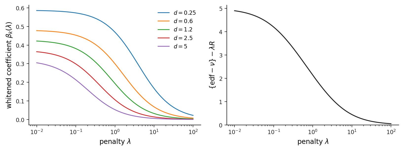
The divergence is a consequence of the mixture geometry, not evidence that the data contain no non-affine structure. Rescaling the roughness matrix changes the numerical scale of \(\lambda\), but does not resolve the underlying problem.
For variance-based smoothing, what we actually need is the uncertainty of the fitted estimator. That requires accounting for the variability of the stochastic gradients.
From curvature to estimator precision
Consider a sample-average objective
with population maximizer \(\eta_0\). Define
and
Here \(A\) describes curvature, while \(B\) measures gradient variability. Under the usual conditions for M-estimation,
The precision corresponding to this asymptotic covariance is therefore
on the identifiable parameter space. The pseudoinverse is relevant because the softmax logits have a common-shift direction that does not change the mixture weights.
For a shared encoder fitted to \(n\) independent observations, there are two sources of stochastic variation: differences between observations and Monte Carlo noise conditional on an observation. If \(g(x,u)\) is the stochastic score and \(S\) independent Monte Carlo draws are used per observation, the relevant covariance is
The corresponding precision is
This is the matrix that should enter a smoothing rule intended to control estimator variance, subject to the appropriate regularity and identifiability conditions.
There is also a connection back to sampling. A sampling design that reduces \(B_S\) improves the precision of the estimated parameters, potentially changing the appropriate amount of smoothing. The variance reductions from stratification are therefore relevant beyond the immediate problem of obtaining less noisy gradients.
However, even an accurately estimated sandwich precision cannot answer every regularization question. It can help determine how much smoothing is warranted by estimation uncertainty, but it cannot decide whether we should deliberately change the population optimum to improve some other measure of approximation quality.
That distinction turned out to be important in the numerical experiments.
Distinguishing Variance Smoothing from Population Model Correction
Write the penalized estimator on the average-objective scale as
The quantity controlling the contribution of the penalty relative to the empirical objective is \(\lambda/n\).
Suppose first that \(\lambda_n=O(1)\) as the sample size grows. Then \(\lambda_n/n\to0\), so the penalty disappears from the limiting population objective. This is the usual behaviour of a regularization term whose role is to stabilize a finite-sample estimate.
Now suppose instead that
Under appropriate convergence assumptions, the limiting estimator maximizes
The roughness penalty remains present even with arbitrarily large samples. In other words, the regularization is not merely controlling finite-sample uncertainty. It is defining a different population optimization problem.
This suggests a simple way of diagnosing what a risk-optimal penalty is doing: examine how it scales with the sample size. If the oracle penalty grows proportionally to \(n\), the evidence points toward a persistent population-level effect rather than regularization that disappears as estimation uncertainty vanishes.
A regular Fellner–Schall fixed point behaves differently. If the fitted roughness converges to a positive constant and the effective degrees of freedom converge, the fixed-point relation
implies that \(\lambda_n=O(1)\). Such a selector cannot asymptotically track an oracle satisfying \(\lambda_n^*/n\to c>0\).
This does not make either penalty intrinsically wrong. It means they are optimizing different aspects of the problem.
Technical note Why the ELBO Hessian is not estimator precision The ELBO Hessian is the mixture Fisher information and comes only from entropy. Estimator uncertainty is a sandwich covariance, and a penalty that grows in proportion to the sample size changes the population objective.
In likelihood-based inference, Fisher information is closely associated with the precision of parameter estimates. This makes it natural to use information matrices when selecting smoothing parameters. Variational inference is different in an important respect: the objective being optimized is not generally the log-likelihood of the observations under a correctly specified statistical model.
To see the distinction, consider a fixed-support spline mixture
and write the ELBO as
Why the Hessian depends only on entropy
Differentiating with respect to a mixture weight gives
The target-dependent term is linear in the weights, so its second derivative is zero.
Consequently,
Defining
we obtain
This identity is exact in the weight coordinates. It establishes concavity of the ELBO, but the matrix represents the local geometry of the mixture rather than directly measuring how precisely its parameters are estimated from observations.
The responsibility-covariance interpretation
The distinction becomes particularly clear in logit coordinates.
Let
Define the component-responsibility vector
Since
we can calculate
At a stationary point, the extra terms arising from the second derivative of the softmax transformation vanish, giving
Because the responsibility vector is a probability vector,
This is a property of the mixture’s geometry. It does not represent a count of informative observations or justify treating the ELBO Hessian as an observation-based precision matrix.
What actually determines estimator uncertainty?
Suppose an estimator maximizes
Let \(\eta_0\) denote the population optimum and define
Under standard M-estimation regularity conditions,
Thus, the asymptotic covariance is governed by both the expected curvature \(A\) and the gradient covariance \(B\).
The corresponding precision matrix is
on the identifiable subspace.
In a correctly specified likelihood model, the Fisher information identity can give \(A=B\). In a variational optimization problem, particularly one involving Monte Carlo gradients or model misspecification, that equality cannot simply be assumed.
Why this matters for smoothing
A roughness penalty has the form
in a simple quadratic parameterization, or a corresponding nonlinear expression when the spline weights are produced by an encoder.
A typical effective-degrees-of-freedom calculation uses
If \(M\) is meant to represent parameter precision, using the ELBO Hessian alone can be misleading. The Hessian captures objective curvature but not the full variability of the fitted estimator.
A particularly revealing failure occurs when the mixture Fisher matrix is used directly in a Fellner–Schall update. In the quadratic approximation analyzed above, the identity
implies that the update continues increasing the penalty at every finite value. The resulting tendency toward extreme smoothing follows from the geometry of the mixture, not from evidence that the observed data support an affine density.
The appropriate uncertainty calculation instead requires a sandwich precision matrix that accounts for the stochastic estimation process.
Variance reduction is not the same as changing the population target
There is a final distinction worth making.
Consider a penalized estimator
If \(\lambda=O(1)\), the penalty disappears from the limiting population objective because \(\lambda/n\to 0\).
If instead
the limiting objective becomes
The penalty remains present even with unlimited data. It is changing the population optimization problem rather than merely stabilizing a noisy estimator.
In the exact \(T=2\) IWAE experiment, the RISE-optimal penalties at sample sizes 100, 200, and 400 were approximately 17.0, 34.6, and 70.2. Their ratios to sample size remained close to 0.17.
This behaviour is consistent with a population-correction effect. It also explains why a variance-based smoothing selector should not necessarily recover an oracle chosen using an external metric such as integrated squared error.
The distinction is therefore not simply between one smoothing algorithm and another. It is between two different statistical tasks: estimating an existing objective accurately and deliberately changing that objective to obtain a better approximation under a different criterion.
A small exact IWAE experiment
To investigate this distinction without introducing Monte Carlo noise into the fitted objective, I used a \(T=2\) importance-weighted variational objective evaluated by deterministic quadrature. The variational model had five spline mixture components and a shared affine encoder. Fitting, penalty selection, and evaluation used independent samples, and five seeds were run at each of \(n=100,200,400\).
The external criterion was root integrated squared error,
This is deliberately different from the IWAE objective. The question was not which penalty maximizes the variational bound, but which penalty gives the smallest density error.
The oracle was selected over 40 logarithmically spaced penalties between 1 and 100. The selected values were interior to the grid, and the five-seed medians were as follows.
Each entry is the median ± the standard deviation over five seeds.
| \(n\) | Fellner–Schall \(\lambda\) | RISE oracle \(\lambda^*\) | \(\lambda^*/n\) | RISE gap |
|---|---|---|---|---|
| 100 | 10.48 ± 1.98 | 17.01 ± 1.17 | 0.1701 ± 0.0117 | 0.000526 ± 0.000556 |
| 200 | 13.57 ± 3.92 | 34.55 ± 2.89 | 0.1728 ± 0.0145 | 0.001629 ± 0.000822 |
| 400 | 16.24 ± 0.10 | 70.17 ± 4.28 | 0.1754 ± 0.0107 | 0.002725 ± 0.000231 |
The RISE gap is the evaluation RISE of the Fellner–Schall fit minus that of the oracle-selected fit.
The oracle penalty nearly doubles whenever the sample size doubles. Across the fourfold increase from \(n=100\) to \(n=400\), its log–log slope is approximately \(1.02\):
The penalty grows with the sample size. The per-observation penalty, \(\lambda_n^*/n\), stays near \(0.17\).
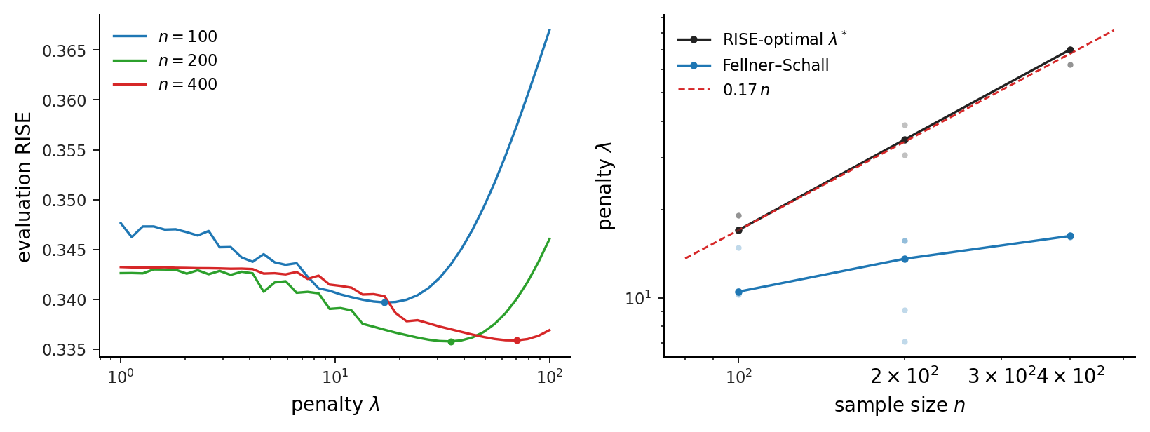
This is the signature of a penalty that continues to modify the population objective. The Fellner–Schall penalty grows much more slowly, so the ratio of its penalty to the RISE-optimal penalty decreases as \(n\) increases.
There are plausible reasons for the external risk to prefer a permanently penalized solution. In a restricted variational family, the population optimum of a \(T=2\) IWAE objective need not be the \(L^2\) projection of the true posterior. The importance-weighted objective has an interpretation involving an augmented or implicit variational distribution, rather than simply reverse KL in the original proposal family.
The affine encoder also introduces its own restriction: even if the spline mixture is flexible for a fixed observation, the shared map \(x\mapsto\gamma(x)\) cannot represent every possible pointwise-optimal mixture. A roughness penalty could compensate for either source of misspecification by moving the fitted model toward a density with lower integrated squared error.
The experiment does not distinguish between these two mechanisms, and the sample-size range is limited. What it does show is that the difference between the two selectors is not appropriately described as the variance-based selector failing to recover the risk oracle. The oracle is choosing a different population fit.
As a further check, selecting the penalty using a held-out version of the unpenalized variational objective produced much smaller penalties, between \(10^{-6}\) and \(0.3\) in the corresponding sweep. That is consistent with the fact that a persistent penalty cannot improve the original population objective over its own unpenalized optimum. It may still improve an external metric such as RISE.
A useful bound for encoder approximation error
There is another observation about the spline mixture that is worth recording because it affects how approximation error scales with the number of basis functions.
Let
We want to understand how an error \(\delta\) in the encoder logits affects the resulting mixture density.
Both \(q_{\widehat\gamma}\) and \(q_{\gamma^*}\) are obtained by marginalizing a joint distribution over the component index and the sample, using the same conditional component densities \(b_k\). The data-processing inequality therefore gives
The discrete KL between softmax vectors is a Bregman divergence of the log-sum-exp function. Bounding its curvature gives
where
The useful feature is that the bound contains no explicit factor involving \(K\), the number of spline components.
If approximation error is measured as an absolute error in every mixture weight, dimension-dependent factors can appear because the individual weights typically shrink as the number of bases increases. Measuring error in logits avoids that issue for this part of the approximation argument. Under the relevant approximation and truncation assumptions, the amortization term can therefore be expressed in terms of squared logit error without an additional factor from the number of basis functions.
This does not remove every form of complexity dependence, and it does not imply unlimited smoothness adaptation. In particular, a penalty based on second derivatives is naturally limited to smoothness adaptation up to order two.
Computational cost and numerical stability
The exact sampler would be less attractive if solving the inverse CDF were prohibitively expensive. Fortunately, most of the cost can be avoided by exploiting spline locality.
In one CPU reference configuration with batch size 128, 16 latent dimensions, 10 samples per dimension, and 24 basis functions, the median timings were:
Median CPU time over five repeats for \((B, J, T, K) = (128, 16, 10, 24)\).
| Sampling method | Median time |
|---|---|
| Local inverse CDF | 35.61 ms |
| Full-basis inverse CDF | 685.85 ms |
| Five-step MH with Concrete relaxation | 1407.62 ms |
| Gaussian draw | 0.0827 ms |
The local implementation was roughly 19 times faster than evaluating the full spline basis during inversion and about 40 times faster than the tested Metropolis–Hastings plus Concrete implementation. Gaussian sampling remained much faster, as one would expect.
The root solver was numerically well behaved in double precision. Safeguarded Newton iteration reached a residual near \(1.11\times10^{-16}\) in eight iterations, while single-precision residuals stopped near \(2.98\times10^{-7}\). For the Fisher information calculations, Gauss–Legendre quadrature with 12 nodes per knot span gave relative errors below \(2.1\times10^{-14}\) in the tested configurations.
There is a related numerical issue in smoothing calculations. Effective degrees of freedom can be evaluated through
where \(d_k\) are generalized eigenvalues of the penalty relative to the information matrix. This representation was stable and monotone even at very large penalty values, whereas direct matrix solves could suffer from cancellation.
As a check on the restricted-likelihood calculations, a Gaussian penalized-spline regression produced a smoothing parameter of \(0.30652445\), compared with \(0.30652447\) from mgcv 1.9-4. That agreement validates the numerical calculation in the regular Gaussian setting; it does not establish that the same information identity holds for a variational objective.
What this means
The main practical result is that spline mixtures are easier to work with than their sampling formulation initially suggests. Their CDF has a simple representation in terms of cumulative mixture weights, which gives an exact reparameterization without introducing a discrete relaxation or running an inner Markov chain. Combined with implicit differentiation, this provides pathwise gradients for the original variational family rather than for an approximation to it. The numerical experiments also show that the resulting one-dimensional transport is particularly well suited to randomized stratification, with substantially lower gradient variance at the same sampling cost.
There are still computational and modeling trade-offs. Inverse-CDF sampling is more expensive than Gaussian reparameterization, and the experiments here are limited to reference problems rather than large-scale generative models. Moreover, the construction does not change the expressiveness of the underlying variational family: the mean-field assumption and compact support remain. What it does establish is that the difficulties associated with sampling from this family need not be addressed by changing the distribution itself.
The analysis of smoothing parameters raises a somewhat different issue. Although the ELBO Hessian has an exact Fisher-information representation, this curvature comes entirely from the entropy term and cannot, by itself, quantify the sampling uncertainty of the fitted parameters. That uncertainty depends on the covariance of the estimating gradients, which is why the sandwich precision is the relevant object for variance-based smoothing. Even with the correct precision matrix, however, there is an important distinction between reducing estimation variance and deliberately changing the population fit. The exact IWAE experiment illustrates this: the RISE-optimal penalty grows approximately as \(\lambda_n^*\approx 0.17n\), so its effect does not disappear as the sample size increases. It is correcting a population-level mismatch rather than simply stabilizing a noisy estimate.
What I find interesting is that both results come from examining assumptions that are easy to take for granted. The use of a Concrete relaxation implicitly accepts that changing the sampling distribution is necessary for differentiation, while directly applying a Fisher-based smoothing rule assumes that objective curvature represents estimator precision. Neither assumption holds in the form needed here. In the first case, exploiting the algebraic structure of the spline family removes the approximation altogether. In the second, examining the source of the curvature reveals why a seemingly reasonable automatic smoothing procedure can fail, and why even a statistically appropriate variance-based selector need not agree with an oracle defined by a different loss.
The broader point is not that approximations or regularization should be avoided, but that their effects need to be separated. Sampling error, estimation uncertainty, and population objective mismatch are different problems, even when they ultimately appear through the same quantity, such as the quality of a fitted posterior. For spline variational families, exact transport makes the sampling problem considerably cleaner. It also gives us a better starting point for studying the remaining questions about how accurately the variational parameters can be estimated and what kind of regularization actually improves the approximation we care about.
Cite this work
If you use this note, please cite it as
De, A. (2026). Exact Reparameterization of B-Spline Mixtures for Variational Inference. Research blog post. https://ananyapam7.github.io/blog/2026/exact-reparameterization-b-spline-variational-inference/
@misc{de2026splinevi,
  author       = {De, Ananyapam},
  title        = {Exact Reparameterization of {B}-Spline Mixtures for Variational Inference},
  year         = {2026},
  month        = nov,
  howpublished = {Research blog post},
  url          = {https://ananyapam7.github.io/blog/2026/exact-reparameterization-b-spline-variational-inference/},
  note         = {Accessed: 2026-11-03}
}
References
Shao, Yu and Feng (2024), Nonparametric Automatic Differentiation Variational Inference with Spline Approximation.
Figurnov, Mohamed and Mnih (2018), Implicit Reparameterization Gradients.
Maddison, Mnih and Teh (2017), The Concrete Distribution: A Continuous Relaxation of Discrete Random Variables.
Durkan et al. (2019), Neural Spline Flows.
Burda, Grosse and Salakhutdinov (2016), Importance Weighted Autoencoders.
Cremer, Morris and Duvenaud (2017), Reinterpreting Importance-Weighted Autoencoders.
Domke and Sheldon (2018), Importance Weighting and Variational Inference.
White (1982), Maximum Likelihood Estimation of Misspecified Models.
Wood and Fasiolo (2017), A Generalized Fellner–Schall Method for Smoothing Parameter Optimization with Application to Tweedie Location, Scale and Shape Models.
Enjoy Reading This Article?
Here are some more articles you might like to read next: