On Variational Inference
A gentle introduction which will take you up to speed with the current research
Start with an observation. Build a target. Fit a distribution.
Prerequisites: probability densities, expectations, and basic calculus.In Bayesian inference, we start with observed data, \(x\), and quantities we do not know but want to learn about, \(z\). These unknowns might be regression coefficients, missing labels, hidden states, or an entire function. How should observing \(x\) change what we think is plausible about \(z\)?
What is unknown, and what is a model?
Imagine measuring a quantity with a noisy instrument. We see the readings, but not the underlying value without measurement error. Different underlying values could plausibly have produced the same readings. Reporting just one guess would hide that uncertainty.
A statistical model specifies a collection of possible probability distributions for the observations. A Bayesian model also describes uncertainty about the unknown quantities, giving a joint probability model for the observations and unknowns. This makes our assumptions explicit: how readings vary around an underlying value, for example, and whether measurement errors are independent.
A probability distribution lets us assign different amounts of plausibility to different possibilities and calculate the probability that an unknown lies in a given range. Treating an unknown parameter probabilistically does not mean its physical value must fluctuate; the distribution represents uncertainty about it. For a continuous quantity, probabilities are areas under a density, rather than the height of the density at a single point.
We will use one notation convention throughout:
| Symbol | Meaning in this article |
|---|---|
| \(x\) | The observed data, held fixed once observed |
| \(z\) | All quantities we want to infer probabilistically |
| \(\theta\) | Model parameters or settings treated as fixed during this inference problem |
| \(\phi\) | Parameters of a variational approximation, introduced later |
Here, an unknown regression coefficient belongs in \(z\) if we want a posterior over it. A known noise level can belong in \(\theta\); if we instead want to infer that noise level, we include it in \(z\). The distinction is what we treat as unknown, rather than whether a quantity is called a parameter or a latent variable.
How a Bayesian model turns observations into an update
We need two ingredients. A prior distribution, \(p_\theta(z)\), describes uncertainty about \(z\) before conditioning on the observed data. A sampling distribution, \(p_\theta(x\mid z)\), describes how observations could vary for a given \(z\), under the fixed settings \(\theta\).
Before observing data, the sampling distribution is a distribution over possible observations. After we observe \(x\), we hold it fixed and view the same expression as a function of \(z\). In that role, it is called the likelihood. A likelihood is not generally a probability distribution over the unknown quantities.
Return to the noisy instrument. For each possible true value, ask how compatible it is with the reading we observed. The likelihood gives more weight to values that make that reading plausible and less weight to values that make it surprising. Multiplying by the prior reweights our initial uncertainty using this compatibility with the data. Normalization then turns the resulting weights into a probability distribution.
Those two ingredients specify one joint distribution. The probability product rule lets us write it in two ways:
Rearranging gives Bayes’ rule. The posterior \(p_\theta(z\mid x)\) is the updated distribution over \(z\), obtained by multiplying the prior by the likelihood and dividing by the evidence \(p_\theta(x)\).
For the interactive example, let the prior be \(z\sim\mathcal N(0,1)\) and the observation model be \(x\mid z\sim\mathcal N(z,0.8^2)\). Completing the square gives
The posterior mean lies between the prior mean and the observation. Its variance is smaller than the prior variance. Moving the observation changes the center; the fixed observation noise keeps the posterior spread constant.
Let the data move your belief
A standard normal prior meets one observation with noise standard deviation 0.8.
The prior favors values near zero; the observation favors values near the measured reading. The posterior balances the two, giving more influence to the more precise source. A more precise measurement would pull the posterior mean closer to the observation and reduce its uncertainty. This slider changes only the reading, while keeping its precision fixed.
In \(\mathcal N(m,s^2)\), the second argument is the variance; \(s\) is the standard deviation. Here the prior variance is \(1\) and the observation-noise variance is \(0.8^2=0.64\), so the observation receives slightly more weight.
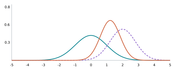
Figure 1. The prior and likelihood are functions of the same \(z\). Multiply them pointwise, then rescale the product to have area one. In this illustration, the posterior shifts toward the values favored by the data.
The joint notation works across models because it leaves open what’s inside each factor. In regression, \(z\) can be a vector of coefficients and we can condition on known inputs. In a state-space model, \(z\) can be a trajectory whose successive states depend on each other. In a mixture model, \(z\) can contain both unknown group labels and continuous group parameters. The update is the same. Only the assumptions that specify the joint probability are different.
From Bayesian inference to a more general inference problem
We have seen that Bayesian inference gives us a posterior distribution over the unknown quantities \(z\), conditional on the observed data \(x\). For continuous \(z\), Bayes’ rule gives
At first glance, this seems to solve our problem: we have an expression for the posterior we wanted. But writing down a distribution and being able to compute or work with it are different things.
In many models, evaluating the joint density \(p_\theta(x,z)\) at a particular value of \(z\) is straightforward. The denominator requires integrating over every possible value. For simple models, this integral may be available analytically. For more complicated models, particularly when the unknowns are high-dimensional and dependent, it can be computationally intractable.
We therefore often know the posterior only up to a proportionality constant:
This suggests a more general formulation. Suppose we are given a nonnegative function \(\gamma(z)\), and we want to work with the probability distribution
We assume \(0\lt Z\lt\infty\), so the target is well defined. Here, \(\gamma\) is the unnormalized density, \(\pi\) is the normalized target density, and \(Z\) is the normalizing constant. For discrete variables, we replace the integral with a sum.
The Bayesian case fits this notation exactly:
Computing a Bayesian posterior is thus one instance of the broader problem of working with a probability distribution specified only up to normalization.
Why is this formulation more general?
The function \(\gamma\) need not come from a prior and a likelihood.
In statistical physics, we may start with an energy function \(U(z)\) for a system in state \(z\). Its Boltzmann distribution at temperature \(T>0\), in units where Boltzmann’s constant is one, is
Here, \(\gamma(z)=\exp[-U(z)/T]\). We do not need an observed dataset or a Bayesian posterior to define this target.
In an energy-based model, an energy function \(U_\theta(z)\) similarly assigns relative plausibility to configurations:
Lower energy means higher density relative to other configurations.
A Gibbs-type distribution can instead combine a reference density \(p_0(z)\) and a loss function \(R(z)\):
Values with smaller loss receive more weight relative to the reference density. The loss need not arise from a likelihood.
These constructions start with different objects: a joint density, an energy function, or a loss. Yet each leads to a target of the form \(\pi\propto\gamma\). This separates defining the probability distribution from performing inference with it.
Different heights. The same distribution.
Multiply a two-peaked density by a constant. Its normalized shape stays put.
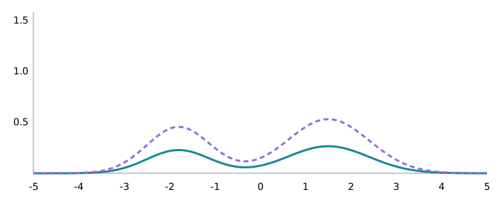
Figure 2. Multiplying \(\gamma\) by a positive constant changes its height and total area by the same factor. After normalization, the target \(\pi\) remains unchanged.
How can we solve the inference problem?
We can evaluate \(\gamma\), perhaps only up to a multiplicative constant, and want to characterize the corresponding target \(\pi=\gamma/Z\). Depending on the problem, this might mean obtaining its density, drawing samples from it, or constructing a tractable approximation to it. These are different kinds of answers to the same underlying inference problem.
Even knowing \(Z\) does not necessarily make integration, marginalization, or sampling easy. Evaluating a density pointwise and performing inference with it are different tasks; the structure of the target determines which methods are practical.
Why knowing the normalizing constant is not enough
Even if the normalizing constant \(Z\) were known, working with the resulting distribution could still be difficult. Knowing the density at any point is not the same as being able to calculate how much probability lies in a whole region. This distinction becomes particularly important when \(z\) is high-dimensional.
Suppose we know \(Z\) exactly and can evaluate \(\gamma(z)\). Then we can evaluate \(\pi(z)=\gamma(z)/Z\) at any chosen point: the normalization problem is solved. But an event probability and a marginal density still require integration:
Here \(B\) is a region of the state space, and \(\pi_1\) is the marginal density of the first coordinate. Computing means and covariances also requires integrals.
A concrete example. Consider the target on \(\mathbb R^d\)
Suppose someone gives us its exact value. Evaluating the density at a chosen vector \(z\) is now straightforward. Yet the marginal density of \(z_1\) is
For each fixed \(z_1\), this is still a \((d-1)\)-dimensional integral. The off-diagonal entries of \(A\) create cross terms because
For a general dense \(A\), these terms couple the coordinates, so the integrand does not factor into a product of one-dimensional functions. It gives us the value of one particular integral over the whole space, not all the partial integrals needed for marginals or event probabilities.
Sampling is a separate problem too. Even if a univariate density is normalized and easy to evaluate, generating a random draw requires a procedure. Inverse-transform sampling provides a theoretical construction:
Constructing the CDF already requires integration, and evaluating its inverse may require numerical work. Sampling becomes harder in higher dimensions. This is why rejection sampling and MCMC can be useful even for a normalized target.
Some distributions are easier because of their mathematical form. For \(\pi(z)=\mathcal N(z;\mu,\Sigma)\), with positive-definite \(\Sigma\), the Gaussian structure gives us moments, marginals, and conditionals, as well as a sampling construction: if \(LL^\top=\Sigma\) and \(\varepsilon\sim\mathcal N(0,I)\), then \(z^\star=\mu+L\varepsilon\) has the target distribution. This tractability comes from the Gaussian family, not simply from knowing its normalizing constant.
The broader problem is therefore how to work with a distribution that may be easy to evaluate pointwise but difficult to integrate, marginalize, or sample from efficiently. Exact methods, Monte Carlo methods, and variational inference address different aspects of this problem.
Exact inference
Some models allow an analytic answer. For example, a Beta prior for a Bernoulli success probability gives a Beta posterior after observing successes and failures. The Gaussian update above is another example: we obtained the posterior mean and variance directly.
Numerical integration and direct sampling
When symbolic calculations are unavailable, numerical integration can approximate the needed integrals. Quadrature can be effective in low dimensions, although the cost of straightforward grid-based methods grows rapidly with dimension.
Alternatively, we may be able to generate independent samples from the target. Rejection sampling is one option if we have a proposal density we can sample from and a suitable bound on the unnormalized target relative to that proposal. It can avoid evaluating \(Z\), but finding a useful bound and achieving a reasonable acceptance rate may be difficult.
Markov chain Monte Carlo (MCMC)
MCMC constructs a Markov chain with \(\pi\) as its stationary distribution. It does not generally compute \(Z\), provide an explicit normalized density, or produce independent draws.
Target-density ratios cancel the unknown normalizing constant, which lets methods such as Metropolis-Hastings construct transitions without evaluating it. Under suitable convergence conditions, the chain approaches the target distribution. Finite runs can explore slowly, and successive samples are generally correlated.
How do MCMC samples answer questions about the target?
For a function \(f\), the expectation \(\mathbb E_\pi[f(z)]\) is its probability-weighted average. A well-mixing chain lets us estimate it by averaging over its samples:
Choosing \(f(z)=z\) estimates a mean; choosing \(f(z)=\mathbf 1_A(z)\) estimates an event probability; choosing \(f(z)=z^2\) estimates a second moment. The indicator is one inside \(A\) and zero outside it. For scalar \(z\), the variance is \(\mathbb E_\pi[z^2]-(\mathbb E_\pi[z])^2\).
Different questions, same distribution
The target stays fixed: a standard normal distribution with mean zero and variance one.
The distribution π(z)
The weighted function f(z)π(z)
Mean: E[z] = 0. Negative and positive contributions cancel. For this same distribution, P(−1 ≤ z ≤ 1) ≈ 0.6827 and E[z²] = 1.
The visual shows exact Gaussian expectations, not a simulated MCMC run. The density stays fixed while the function being averaged changes. The second moment equals the variance here only because the mean is zero.
Variational inference
Variational inference (VI) introduces a family of tractable distributions \(q_\phi(z)\), indexed by parameters \(\phi\), and fits a member of that family to the target:
For example, suppose we allow only Gaussian approximations, \(q_\phi(z)=\mathcal N(z;m,s^2)\), with \(\phi=(m,s)\) and \(s>0\). We can move the center and change the spread, but every candidate remains Gaussian. The parameters \(\phi\) are the controls for those adjustments; fitting the approximation means choosing their settings. This family is tractable because we can evaluate its density and generate samples easily.
A single Gaussian cannot reproduce every target: it cannot match two separated peaks exactly, however carefully we adjust its center and spread. Choosing the family determines which shapes are available; optimization chooses among those shapes.
The result is a fitted distribution that we can use to describe uncertainty and calculate or estimate quantities of interest. Its accuracy depends on both what the family can represent and how well we optimize within it.
What does it mean for one distribution to approximate another well? We need a criterion that compares their probability assignments, and a family in which we can optimize that criterion.
A common choice is reverse Kullback-Leibler divergence:
Imagine drawing values from our current approximation. At each draw, compare the density assigned by the approximation with the density assigned by the target, using their log ratio. Reverse KL averages this comparison over the places the approximation itself visits. Changing the direction of KL changes whose draws we average over.
KL is nonnegative and is zero when the two distributions match. It is not a symmetric distance: exchanging \(q_\phi\) and \(\pi\) changes the criterion.
Why this direction? The expectation is taken under our own approximation, which we choose to make tractable. We can often sample from \(q_\phi\) and evaluate its density even when we cannot directly sample from \(\pi\). The criterion also strongly penalizes putting mass where the target has very little density. Other divergence criteria are possible, and this choice affects which approximation is preferred.
Why can reverse KL favor just one of two peaks?
The two animations show a two-dimensional target with two separated modes. Blue contours stay fixed; the red Gaussian approximation moves and changes shape. Forward KL stretches the red contours across both modes, while reverse KL tightens them around one.
For a precise description, write the target in coordinates \(w=(u,v)\):
The plots rotate both distributions by 25 degrees, \(z=Rw\), to place the modes diagonally. This shared rotation changes neither KL objective. Both runs start at \((m_u,m_v)=(1.2,-1)\) and \((s_u,s_v)=(1.3,1.8)\). Only the direction of KL changes:
Same starting point, different destinations
Blue contours show the fixed two-mode target. Dashed red contours show the Gaussian moving and changing shape as its KL decreases. The red dot marks its center.


Forward KL asks whether the approximation covers places the target visits. The target visits both peaks. A narrow Gaussian on one peak would assign extremely small density to draws from the other, producing a large penalty. The fitted Gaussian therefore broadens to cover both. For this target, the forward-KL optimum matches its mean and covariance: in the unrotated coordinates, \((m_u,m_v)=(0,0)\) and \((s_u^2,s_v^2)=(9.36,0.64)\). It covers both peaks, but also puts substantial probability in the valley: a single Gaussian cannot reproduce the target’s two-peak shape.
Reverse KL asks whether the places the approximation visits are plausible under the target. A broad Gaussian visits the valley between the peaks, where the target density is tiny. Narrowing around one peak avoids those visits. Once the approximation concentrates there, it rarely visits the other peak, which receives little direct weight in the expectation. Here the run settles near \((m_u,m_v)=(3,0)\) and \((s_u,s_v)=(0.6,0.8)\), matching the upper-right component after rotation.
The target is symmetric, but the starting approximation is offset toward the positive-u mode. That offset selects the upper-right solution in this run; reflecting the initial u-coordinate would select the other mode. The available shapes matter too: a family with two Gaussian components can represent this particular target exactly.
The loss plots show improvement within each run. Their numerical values measure different objectives and should not be compared as a single ranking of the two fits.
With a chosen family and criterion, we seek
In practice, optimization may find a local optimum.
There is an apparent obstacle: the objective contains \(\pi\), whose normalizing constant may be unknown. But substituting \(\pi=\gamma/Z\) turns that unknown scale into an additive \(\log Z\). For a fixed target, this term is the same for every candidate, so it does not affect which variational parameters optimize the objective. Computing the numerical KL value and optimizing it are therefore different requirements.
Let us make that cancellation explicit, one step at a time.
From reverse KL to the ELBO
Keep the target fixed while we vary \(\phi\), with \(q_\phi\) a normalized density.
Start with the reverse KL we want to minimize:
Because \(\pi(z)=\gamma(z)/Z\), we have \(\log\pi(z)=\log\gamma(z)-\log Z\). Substituting, and keeping track of the minus sign, gives
The logarithm has turned the unknown multiplicative scale into an additive term. We have not computed \(Z\); we have isolated where it enters the objective.
For this fixed target, \(\log Z\) does not depend on \(z\). Since \(q_\phi\) integrates to one,
So, even though the averaging distribution changes with \(\phi\), this particular expectation stays constant. We obtain
Reverse the signs inside the remaining expectation and define
There is also an intuitive way to read these two terms:
The first term rewards putting probability in regions where the target density is high. The entropy term rewards retaining spread. Together, they balance concentrating in plausible regions with representing uncertainty, rather than simply selecting one high-density point. Spreading out indiscriminately is not rewarded overall: it can move probability into regions with low target density and worsen the first term.
A note on entropy for continuous distributions
For continuous distributions, \(\mathcal H\) is called differential entropy. For a Gaussian, \(\mathcal H(\mathcal N(m,s^2))=\tfrac12\log(2\pi e s^2)\), so increasing its spread increases its entropy. Shrinking its spread to zero drives that entropy to minus infinity.
This quantity is the evidence lower bound, or ELBO, when our target is a Bayesian posterior. The same objective also applies to a general unnormalized target. Substitution gives the central identity:
Notice what the ELBO requires: evaluations of \(\log\gamma\), evaluations of \(\log q_\phi\), and an expectation under \(q_\phi\). It does not require the value of \(Z\).
For a fixed target, \(\log Z\) is a fixed level. The ELBO sits below it, and the distance between them is exactly the reverse KL. If we raise the ELBO by one unit, the KL falls by one unit:
Therefore the same parameters solve both optimization problems:
We do not need to know the height of the fixed level to move toward it. Comparing ELBO values is enough to tell which candidate has the smaller reverse KL.
Close the gap
Fit a Gaussian to a Gaussian target. Every unit gained in ELBO removes one unit of KL.
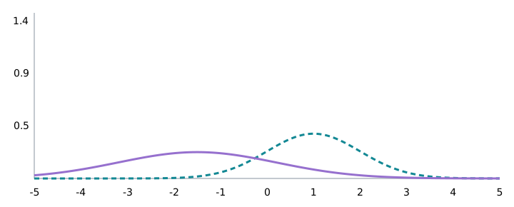
Dashed line: fixed \(\log Z\). Violet line: ELBO. Shaded gap: reverse KL. Both lines use the same fixed vertical scale.
In this illustration, the target is \(\pi=\mathcal N(1,1)\), the approximation is \(q_{m,s}=\mathcal N(m,s^2)\), and we deliberately choose \(\gamma=e^2\pi\), so \(\log Z=2\). The Gaussian KL has the closed form
Move the mean or spread and watch both views: the approximation changes shape above, while the ELBO and its gap to \(\log Z\) change below. At \(m=1,s=1\), the densities agree and the gap closes. The play button smoothly moves to this known solution; it illustrates the identity rather than running a general-purpose optimizer. The fixed value of \(\log Z\) is shown because this example is solvable, not because VI normally knows it.
KL divergence is nonnegative, so the identity immediately implies
In the Bayesian case, \(\gamma(z)=p_\theta(x,z)\) and \(Z=p_\theta(x)\). Consequently,
The ELBO is thus a lower bound on the log evidence. Equality holds when \(q_\phi\) matches the posterior. If the variational family cannot represent the posterior, even its best member leaves a gap. An imperfect optimization procedure can leave an additional gap.
The identity removes the need to compute the normalizing constant, but we still need to evaluate or estimate the ELBO and optimize it. This is where the research begins: what is the smallest change that makes the next problem tractable?
A connected reading of variational inference
Each entry makes two things explicit: the setup it assumes and the contribution it makes. A factorization of the model describes how the unknowns and observations depend on one another. A factorization of \(q_\phi\) describes the approximation we choose. These are different decisions.
From there, a paper may change the approximation family, the objective, the gradient estimator, or the optimization procedure. Others analyze an existing method’s error or convergence. Keeping these distinctions separate lets us see which ideas can be combined: a richer family can use a better gradient estimator without changing the target. Follow the questions below, or the connections beside each paper.
We keep \(x\) for observations, \(z\) for unknowns, \(\theta\) for model parameters, and \(\phi\) for approximation parameters. Throughout,
The importance weight \(w_\phi\) compares the unnormalized target with the approximation at a sampled point. It will connect ordinary VI to several alternative objectives. In the notes, \(q\) and \(w\) abbreviate \(q_\phi\) and \(w_\phi\); \(\epsilon\sim\nu\) denotes base noise, and \(\widehat g_\phi\) a sampled gradient. Each new symbol is introduced where it is needed.
When a paper learns the model as well as the approximation, we write the Bayesian specialization \(\gamma(z)=p_\theta(x,z)\). An inference update varies \(\phi\) while holding \(\theta\) fixed.
Shared notation for the paper notes
\(q_j=q_{\phi_j}\) denotes a factor, and \(q_{-j}=\prod_{k\ne j}q_k\) the remaining factors. Parenthesized superscripts mark optimization iterates: \(q^{(t)}\) and \(\phi^{(t)}\). A star denotes an optimum; a hat denotes an estimate.
Samples are \(z^{(s)}\), with importance weights \(w_s=w_\phi(z^{(s)})\) and normalized weights \(\bar w_s=w_s/\sum_r w_r\). We use \(K\) for the number of Monte Carlo draws, \(N\) for observations, and \(d\) for dimension.
\(\mathcal L[q]\) views the ELBO as a functional of a distribution; \(\mathcal L(\phi)=\mathcal L[q_\phi]\) views the same quantity as a function of its parameters. Gaussian factors use mean \(m_j\), standard deviation \(s_j\), and variance \(v_j=s_j^2\). Optimization step sizes are \(\eta_t\); \(\rho\) denotes correlation. Additional parameters for a learned control variate use \(\psi\).
No matching papers. Try a method name, author, or year.
How do we actually optimize the ELBO?
Start with a choice of approximation family and an optimizer. Then distinguish the model structure a paper assumes from the inference machinery it introduces.
Mean-field variational inference (MFVI)
Source paper: A Mean Field Theory Learning Algorithm for Neural Networks
The move. Choose a tractable family by separating the unknowns into independent blocks.
Read with CAVI · Normalizing flows · Hierarchical VI
The idea and the mathematics
A flexible joint approximation can be expensive to store, sample, and optimize. Mean field starts with a simpler choice: represent uncertainty in separate blocks.
The idea is to simplify dependence. Instead of fitting one unrestricted joint distribution, choose independent blocks:
We abbreviate each factor as \(q_j\). Under \(q_1(z_1)q_2(z_2)\), drawing a large \(z_1\) does not make a large \(z_2\) more likely. Each block can still contain several dependent unknowns; independence is imposed between blocks.
This makes sampling and density evaluation simple: draw each block separately and add their log densities. The target still couples the optimization problems, so the best choice for one factor depends on the others. MFVI chooses the family; CAVI or gradient methods choose its parameters.
The cost is lost geometry. A correlated Gaussian has tilted contours, whereas a product of scalar Gaussians has axis-aligned contours.
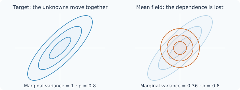
For example,
The true marginal variances are \(1\), but at \(\rho=0.8\) the fitted variances are \(0.36\). Widening independent factors would put mass outside the narrow tilted region, so reverse KL favors a narrower approximation.
When it helps. Mean field offers inexpensive inference when dependencies are weak or speed matters. Strong correlations can make uncertainty too narrow, and separated modes can lead to a fit around just one mode. Larger blocks, flows, or hierarchical approximations can retain more structure.
The independence assumption belongs to the approximation \(q_\phi\), not to the target \(\pi\). The featured Peterson–Anderson paper uses mean-field equations and factorized correlations to replace expensive sampling during Boltzmann-machine learning. The broader MFVI idea below is a choice of approximation family; the model and reverse-KL objective stay fixed.
Coordinate-ascent variational inference (CAVI)
Source paper: Mean Field Theory for Sigmoid Belief Networks
The move. Optimize one factor at a time, using the current distributions of all the others.
Read with SVI · BBVI · Linear-response covariance
The idea and the mathematics
Once we have chosen independent variational factors, we still need to fit them. Each factor's best setting depends on the others, suggesting an alternating procedure.
The idea is to improve one distribution at a time. Starting from a mean-field approximation, freeze every factor except one and choose its best replacement. Then move to the next factor using the latest versions of all the others.
Write \(q_{-j}=\prod_{k\ne j}q_k\). The core update is
For each possible value of \(z_j\), average the log target over our current uncertainty about the other blocks. Exponentiate and normalize to obtain the updated factor. We average over the other distributions rather than fixing their unknowns at single values.
Why it works. This is the exact maximizing factor when the displayed distribution is available in the chosen family. With every other factor fixed, it cannot lower the ELBO:
Here \(t\) counts individual factor updates. A complete pass through the factors is a sweep. Each step replaces a whole distribution, including its spread.
A concrete example. For the correlated Gaussian in the MFVI section, the updates alternate as
Each mean follows the current mean of the other factor. The second update uses the first factor's newly updated mean. Watch one marginal move while the other stays fixed:
One factor moves. The ELBO climbs.
Blue contours are the target. Orange contours are the current product approximation. The marginal plots show each factor in orange and its true target marginal in dashed blue. Each button press performs one exact factor update.
Start with q₁; q₂ stays fixed.
Enable JavaScript to step through the factor updates.
Where it struggles. The expectation and normalization must be tractable; conditional conjugacy often makes this possible. Otherwise, BBVI offers estimated gradients. Strong coupling can slow the alternating updates, and general objectives can have poor local optima. Even perfect convergence cannot recover dependence excluded by mean field. SVI addresses the separate cost of processing a large dataset per update.
CAVI is an optimization strategy for a factorized approximation: it changes which factor is optimized at each step, while keeping the target and ELBO fixed. The featured Saul–Jaakkola–Jordan paper applies bound ascent to sigmoid belief networks, using Bernoulli mean-field factors and auxiliary bounding parameters to handle their nonlinear conditionals. The general update below describes exact coordinate maximization; that paper's extra bound is needed when the model does not make this update tractable.
Stochastic Variational Inference
The move. Replace the full-data coordinate update with a minibatch estimate of its natural-gradient direction.
Read with CAVI · BBVI · Joint control variate
The idea and the mathematics
In a large dataset, a coordinate update for a shared unknown may require fitting a local factor for every observation. SVI reduces that cost by learning from a small batch at a time. To see how, we first need a model whose contributions can be separated by observation.
First, the model supplies the decomposition. Split our unknowns as \(z=(z_g,z_1,\ldots,z_N)\), where \(z_g\) is shared and \(z_i\) belongs to observation \(x_i\). The joint density has the form
Given the global unknown, the observation–local-variable pairs separate. In a topic model, the topics are global, while each document has its own topic proportions and assignments. This is an assumption about how the data are generated.
We approximate the posterior using a global factor and one factor for each observation:
This is a separate assumption: the approximation makes the global block and the local blocks independent, even though the posterior generally couples them.
The factorization tells us which distributions to fit, but not whether their updates are computable. The original SVI construction therefore focuses on models with conditionally conjugate exponential-family distributions. We can unpack this requirement in two steps.
An exponential family expresses a density through a fixed collection of functions of its variable, with adjustable coefficients. We choose the global variational factor in the form
Here \(T_g\) collects sufficient statistics, \(\phi_g\) is their coefficient vector (the natural parameter), \(h\) is a fixed base measure, and \(A\) is the log normalizer that makes the density integrate to one. For a Gaussian, the statistics are \(z_g\) and \(z_g^2\), and the natural parameters are \(m_g/v_g\) and \(-1/(2v_g)\). So averaging natural parameters is generally different from averaging means and variances.
Conditional conjugacy means that conditioning on the other unknowns and the observations leaves the global variable in the matching family. This conditional distribution is called its complete conditional. In the model class considered here, it has the form
Here \(\alpha_0\) is the prior natural parameter and \(T_i(x_i,z_i)\) is observation \(i\)'s contribution to it. In the CAVI update, taking the expectation over the local factors only changes the coefficients: \(T_i\) becomes \(\bar T_i=\mathbb E_{q_i}[T_i(x_i,z_i)]\). The functional form survives. That is why a whole distribution update reduces to adding a few expected statistics. The vector \(T_i\) includes any count terms needed by the conjugate family. Matching exponential-family local conditionals likewise makes local coordinate updates tractable; a local block may still require several such updates.
CAVI can now require a pass through every observation before updating the global factor. In natural-parameter coordinates, its global optimum for fixed local factors takes the form
The full-data update is thus the prior contribution plus all the fitted local contributions.
Each local contribution depends on the current global belief. We therefore hold the global factor fixed and fit the local factors before collecting their expected statistics. Conceptually, this gives an objective depending only on the global parameters:
In the document example, each local fit uses the current global topic distribution before contributing its expected word counts. At an exact local optimum, the local first-order derivatives vanish, so the global derivative can be evaluated holding those optimized local parameters fixed. We do not need to differentiate through every local optimization step.
To turn these best responses into an optimization direction, SVI uses a natural gradient: a gradient adjusted for how parameter changes alter the distribution. The Fisher information matrix \(I(\phi_g)\) measures this local geometry. For our exponential-family factor,
This is the second place the exponential-family structure pays off: the ordinary gradient contains exactly the Fisher matrix. The natural gradient cancels that matrix, leaving
A minibatch estimates the whole sum. For a uniformly sampled batch \(\mathcal B\), rescale its contribution:
At iteration \(t\), \(\bar T_i^{(t)}\) uses the current local fit, and \(\widehat\phi_g^{(t)}\) is the resulting minibatch proposal.
The factor \(N/|\mathcal B|\) puts a small batch on the scale of the full dataset. The step size \(\eta_t\) prevents one noisy batch from replacing everything learned so far.
The minibatch update estimates that direction. Compared with CAVI on this same model and family, the objective and model structure remain; the expensive full-data update becomes stochastic. BBVI introduces a different source of randomness: draws of the unknowns from \(q_\phi\). SVI's conjugate expectations can be computed analytically, so stochastic optimization here need not involve sampling the latent variables at all. Joint control variates address both sources together.
Think of each local fit as a message to the global fit. In a topic model, a document's local factors describe which topics explain its words. Their expected word counts become evidence for the shared topics. A minibatch sends only a few such messages, scaled up to estimate the messages from the whole corpus. Repeating this over different documents builds a global picture without rereading the entire corpus at every step.
The natural gradient makes the connection to CAVI particularly clean: it points from the current natural parameter toward the coordinate optimum. A full step with all observations recovers that coordinate update; a smaller stochastic step moves toward an estimated optimum. The geometry matters because equal changes in a distribution's raw parameters need not represent equal changes in the distribution.
A few local fits move one global belief
Follow four stages: select three observations, fit their local factors, send scaled statistics, then blend the global natural parameters. Teal is the current global approximation; dashed blue is the best global factor in this mean-field family.
- Select batch
- Fit locals
- Scale messages
- Update global
The small model behind this animation
We use twelve fixed observations and a conjugate Gaussian model:
With the global mean held fixed, each selected local fit is exactly
Its message is \(\bar T_i=(m_i,-1/2)\). For a batch of three, multiply the sum by \(12/3=4\), add the prior parameter \((0,-1/2)\), and blend with \(\phi_g=(m_g/v_g,-1/(2v_g))\). The step size is \(\eta_t=(t+2)^{-0.7}\), starting at \(t=0\). Batches are sampled uniformly without replacement within each batch, with a fixed random seed for replay.
The dashed density has \(m_g^\star=\sum_i x_i/14\) and \(v_g^\star=1/13\). The ELBO plot evaluates \(\mathcal L_{\mathrm{prof}}(\phi_g)-\mathcal L_{\mathrm{prof}}(\phi_g^\star)\): it analytically refits all local factors for this diagnostic only. The algorithm itself fits just the selected three. This lets us compare global fits on the same full-data objective.
Exponential-family notation alone is not enough. A Gaussian approximation to a nonconjugate model does not automatically give the additive update above. Conjugacy supplies the matching log-density form; the exponential family supplies the coefficient representation and Fisher identity; the global–local decomposition supplies the sum we can subsample.
When this helps. The data must have exploitable local/global structure, and the conjugate updates must be available. The expensive part becomes fitting the local factors for the selected observations. Inaccurate local fits can spoil the gradient estimate; a nonconjugate model does not automatically inherit these closed-form directions. Unlike exact CAVI, an individual noisy minibatch update can lower the ELBO. Progress emerges across updates with a suitable step-size schedule.
The broad idea of stochastic optimization applies much more widely. But using SGD on an ELBO is not enough to inherit this paper's local fitting rule, sufficient-statistic sum, or natural-gradient formula. Those come from the particular model and variational structure above.
Black Box Variational Inference
The move. Replace model-specific coordinate algebra with a score-function estimate of the same ELBO gradient.
The idea and the mathematics
The factor update in CAVI contains an expectation of the log target. When that expectation has no tractable expression, we need a way to improve the ELBO using quantities we can still compute.
BBVI keeps the ELBO and the chosen variational family, but replaces model-specific expectation calculations with score-function Monte Carlo gradients. It needs samples from \(q_\phi\), its log-density derivatives, and evaluations of the log joint; conditional conjugacy is unnecessary. Its practical algorithm combines Rao–Blackwellization and control variates, using mean-field structure to isolate relevant model terms. This randomness comes from latent draws, whereas SVI's minibatch randomness comes from observations.
What if the coordinate expectation cannot be integrated analytically? We can still draw from \(q_\phi\) and estimate a gradient. Define its score
This tells us how the log density at a fixed point changes when we adjust the approximation. Using \(\nabla_\phi q_\phi=q_\phi S_\phi\), differentiate the ELBO:
The last integral vanishes because \(\mathbb E_{q_\phi}[S_\phi]=\nabla_\phi\int q_\phi(z)\,dz=0\). So samples from the approximation give the estimate
The log weight measures how the target and approximation compare; the score tells us how to change the approximation's density at the sampled point. Their product turns the comparison into an update direction.
The estimate can be noisy. The paper reduces this noise with control variates and by averaging out irrelevant variables (Rao–Blackwellization). The new ingredient is an estimated gradient of the same ELBO. AEVB obtains that gradient by moving the samples instead of differentiating their density.
An example of the noise we can remove. Suppose one coordinate of \(z\) explains only a small part of the model, but its score is multiplied by the log joint for everything. Random changes in unrelated terms then perturb that coordinate's update without providing useful information about it. Rao–Blackwellization removes terms whose expected contribution is zero, leaving the relevant local terms. It is a way of asking each factor to respond to the evidence that actually concerns it.
Similarly, for a constant \(b\),
Subtracting a baseline changes the random fluctuations but not their average. A good baseline makes the learning signal describe whether a sample is better or worse than expected, rather than carrying a large common offset.
What black box buys us—and what it costs. We need samples, log-density evaluations, and the variational score, without a hand-derived coordinate update or a derivative of the model with respect to \(z\). This makes discrete variables possible too. But a very noisy learning signal, particularly in many dimensions, can make optimization slow. The estimator also learns only from regions visited by \(q_\phi\); unbiased gradients do not guarantee that a poorly initialized approximation discovers a distant mode.
Auto-Encoding Variational Bayes
The move. Combine pathwise ELBO gradients with an inference network for joint inference and generative-model learning.
Read with BBVI · Stochastic backpropagation · Sticking the Landing · Amortization gap
The idea and the mathematics
A score-function gradient can be computed for many distributions, but its noise can make learning slow. For continuous unknowns, there is another source of information: how a sampled value moves when the variational parameters change.
AEVB addresses differentiable generative models with continuous latent variables and a reparameterizable approximation. It combines two changes: a pathwise ELBO-gradient estimator, and an inference network that shares variational parameters across observations. Jointly learning the generative parameters \(\theta\) and inference parameters \(\phi\) gives the VAE construction. The objective remains the ELBO; neither conditional conjugacy nor closed-form CAVI updates are required.
In BBVI, we differentiate the distribution that produces a draw. Here we express the draw itself as a differentiable function:
When the observation is explicit, write \(q_\phi(z\mid x)\); for fixed \(x\), this is the same \(q_\phi(z)\) used throughout.
The noise law \(\nu\) stays fixed. For a diagonal Gaussian approximation,
Hold the same noise draw while changing \(\phi\). The resulting sample moves smoothly, so ordinary differentiation can follow its movement:
This is a pathwise gradient. It uses the slope of the target along the moving sample, rather than only a density comparison at a fixed point.
The paper also introduces shared inference: a network predicts \(m_\phi(x)\) and \(s_\phi(x)\) for each observation. This is amortization—learning how to infer across many observations. The model parameters \(\theta\) can also be trained; they remain distinct from the inference parameters \(\phi\), and are held fixed when taking the inference gradient above.
Stochastic backpropagation develops a closely related route. Sticking the Landing removes a noisy term from this derivative. Inference suboptimality asks what is lost when an encoder chooses the local approximation.
Follow one draw. For a scalar \(z=m+s\epsilon\) and a fixed smooth function \(f\),
Increasing \(m\) moves every draw right. Increasing \(s\) moves positive-noise draws right and negative-noise draws left. The derivatives ask whether these movements improve the function. For \(f(z)=z^2\), the sampled mean-gradient is \(2(m+s\epsilon)\), whose average is \(2m\). Holding the noise fixed gives a meaningful comparison between nearby parameter settings.
In a VAE, the same mechanism tells the encoder how changing a latent code affects reconstruction. The ELBO balances expected log likelihood against the KL to the prior: useful codes should explain the observation while keeping the approximate posterior compatible with the generative model.
Where the difficulties move. A hard discrete draw does not move smoothly, motivating Concrete and discrete estimators. Even with smooth draws, steep decoder derivatives can produce noisy gradients. And a fast encoder can return a suboptimal local distribution: reparameterization makes its gradient tractable, while amortization-gap methods address how well its output actually solves inference.
Stochastic Backpropagation and Approximate Inference in Deep Generative Models
The move. Develop stochastic backpropagation and recognition models for deep Gaussian latent-variable models.
Read with AEVB · Local reparameterization
The idea and the mathematics
A deep latent-variable model passes uncertainty through several layers before producing an observation. Learning such a model requires gradients that account for how changes in one layer affect the expected behavior of later layers.
This paper develops stochastic backpropagation for deep directed models with Gaussian latent layers. It couples tractable approximate posteriors and recognition networks with gradient identities that differentiate expectations through Gaussian uncertainty. The contribution is a practical inference-and-learning framework for these models, rather than a new divergence. The Gaussian structure supplies the differentiable sampling route; it is a substantive specialization of our generic \(z\).
An independent route to similar gradient machinery starts with Gaussian differentiation identities. Here \(m\) and \(\Sigma\) are the mean and covariance components of \(\phi\). For smooth \(f\) and \(z\sim\mathcal N(m,\Sigma)\),
The first formula moves a derivative with respect to the Gaussian mean onto the function being averaged. A location-scale representation also gives first-order derivatives through a factor of \(\Sigma\). The paper develops these ideas for backpropagation through layers of latent Gaussian variables. AEVB is the simplest entry point for the sampling transformation. This paper makes the Gaussian calculus behind it explicit.
Why the two Gaussian identities make sense. Moving the mean translates the whole cloud, so the average slope of \(f\) determines the change. Changing the covariance spreads the cloud instead. Whether spreading helps depends on curvature: a convex bowl rewards spread in its upward-curving directions, whereas a concave hill penalizes it. For the scalar example \(f(z)=z^2\), we have \(\mathbb E[f]=m^2+v\). The mean derivative is \(2m\), and the variance derivative is \(1=\tfrac12 f''\).
Computing a full Hessian would be expensive in a large latent space. Instead, write \(\Sigma=BB^\top\) and \(z=m+B\epsilon\). Then
This replaces the covariance derivative involving second derivatives with a scale-factor derivative involving first derivatives. Repeating the chain rule through successive latent Gaussian layers makes deep stochastic models trainable with backpropagation.
When it helps. The method is especially natural when Gaussian noise enters smooth neural computations. The Gaussian identities do not directly solve discrete sampling, and a simple Gaussian recognition model may still miss posterior dependencies or multiple modes. This paper supplies gradient machinery; flows later enrich the distributions that machinery can train.
Automatic Differentiation Variational Inference
The move. Transform constrained unknowns to an unconstrained space, then fit a Gaussian with automatic differentiation.
Read with AEVB · Normalizing flows · DADVI
The idea and the mathematics
Even with a usable gradient estimator, implementing VI for a new model can require transformations, derivatives, and distribution-specific code. ADVI aims to automate that work for models with continuous unknowns.
ADVI targets models with continuous unknowns and a differentiable log density. It maps constrained unknowns to an unconstrained space, fits a Gaussian there, and automates pathwise gradients with automatic differentiation. Thus it specifies the approximation family and computational pipeline while retaining the ELBO. The transformation is a change of coordinates, including its density Jacobian; it does not assert that the original posterior is Gaussian.
If \(z\) is constrained, first map it to \(u=T(z)\in\mathbb R^d\). The transformed log unnormalized target is
Fit a diagonal or full-rank Gaussian in \(u\)-space and differentiate its ELBO automatically using reparameterization. The change-of-variables term matters because a Gaussian in \(u\) induces a generally non-Gaussian distribution in \(z\). AEVB learns an inference network for a model class. ADVI uses the same gradient principle to fit a given probabilistic model. DADVI revisits how ADVI handles Monte Carlo draws during optimization.
A positive unknown makes the construction concrete. If \(z\gt 0\), take \(u=\log z\), so \(z=e^u\). The transformed target becomes
The extra \(u\) is the log Jacobian. An interval of width one in \(u\) represents a much wider interval in \(z\) at large \(u\); the Jacobian accounts for that stretching. Omitting it would optimize against the wrong distribution. A Gaussian approximation for \(u\) induces a lognormal approximation for \(z\), so positivity is automatic and skewness is possible even with a Gaussian fitting engine.
ADVI then writes \(u=m+B\epsilon\), differentiates the transformed log target, and estimates its gradient with draws of fixed-law noise. Constraints, derivatives, and stochastic optimization are handled by a common pipeline rather than a fresh derivation for every model.
What automation cannot choose for us. The transformed posterior still needs to be well approximated by the chosen Gaussian. A curved ridge or separated modes may remain difficult after removing constraints; a full covariance captures linear dependence but does not bend a Gaussian around a ridge. Discrete unknowns also lie outside this continuous transformation pipeline. ADVI removes much of the implementation work, not the need to assess the approximation.
Gradient Estimation Using Stochastic Computation Graphs
The move. Combine score-function and pathwise contributions in a single computation graph.
Read with BBVI · AEVB · Gradient estimation survey
The idea and the mathematics
A learning objective may combine ordinary calculations with several random draws. To differentiate its expectation correctly, we need to know which random choices can influence each part of the final cost.
Stochastic computation graphs treat a differentiable expected cost built from deterministic operations and stochastic nodes. VI is one application. The paper gives a graph-based gradient rule combining score terms and ordinary derivatives, with downstream costs determining credit assignment. It changes how gradients are constructed, without prescribing a new posterior family, model factorization, or VI objective.
Factor a computation into conditional draws \(v\sim p(v\mid\mathrm{parents})\) and deterministic operations. Differentiating the joint sampling density gives a score contribution for each stochastic node. Only costs downstream of that node need to multiply its score, since the expected product with an unaffected cost vanishes after conditioning on the appropriate predecessors. Differentiable paths contribute ordinary chain-rule terms. BBVI and AEVB can therefore appear in different parts of the same model. This is especially helpful when the model has both continuous and discrete random variables.
Consider a discrete gate followed by a continuous computation. Draw \(z\sim q_\phi\), compute \(h_\phi(z)\), and evaluate a cost \(c(h_\phi(z))\). There are two ways \(\phi\) changes the average cost: it changes how often each gate is chosen, and it changes the computation after a gate has been chosen. Thus
The first term handles the random choice; the second is ordinary backpropagation. Ignoring the first would never teach the model which choices to make. Including unrelated costs in it would add noise without useful credit assignment.
The paper organizes these rules into a graph-based surrogate whose derivatives produce the desired estimator. This makes mixed stochastic programs easier to implement and explains where baselines can depend on earlier information.
Its scope. This is a framework for constructing correct gradients, not a promise that they have low variance. A long downstream sequence can give a very noisy score signal; a long differentiable path can have exploding derivatives. NVIL, RELAX, and the pathwise methods can be understood as improving particular pieces of this graph.
Monte Carlo Gradient Estimation in Machine Learning
The move. Compare score, pathwise, and measure-valued representations of a derivative under one framework.
Read with BBVI · AEVB · Stochastic computation graphs
The idea and the mathematics
The preceding methods use different routes to differentiate expectations. This survey organizes those routes so that we can choose an estimator based on the information a model and its approximation provide.
This is a survey of Monte Carlo gradient estimation, rather than a proposal for a new VI model or optimizer. Its organizing contribution is to compare score-function, pathwise, and measure-valued derivatives through their assumptions and variance-reduction tools. Read it as a map for deciding which estimator can serve an already chosen objective and approximation family.
The survey distinguishes three representations of the same derivative. The score representation differentiates the density. The pathwise representation moves samples and differentiates the integrand. A measure-valued representation writes a derivative of a probability measure as \(c(\mu^+-\mu^-)\), giving \(c(\mathbb E_{\mu^+}f-\mathbb E_{\mu^-}f)\). The third perspective is especially useful when you can evaluate a function at coupled draws even when the function itself is hard to differentiate. This provides the common vocabulary for comparing BBVI, AEVB, and the discrete estimators below.
A Bernoulli variable connects all three viewpoints. Write \(p=\operatorname{sigmoid}(\phi)\). For a fixed function \(f\),
The score estimator recovers this by randomly choosing an outcome and weighting its function value. A measure-valued derivative represents it directly as the difference between point masses at 1 and 0, scaled by \(p(1-p)\). A naive pathwise derivative through a threshold gives zero almost everywhere and misses the movement of probability across the threshold.
The survey's practical lesson is to choose a representation based on the computation available. Can we differentiate \(f\)? Can we evaluate it at paired samples? Can a baseline remove a large common offset? Is one estimator cheap enough to afford more draws? Its comparisons show why low variance alone is not the whole decision: derivative evaluations, additional function calls, and the behavior of the particular integrand also matter.
How to use this entry. It is a map of the estimator literature, rather than another proposed VI objective. Use it when choosing between the neighboring methods. Smoothness favors pathwise methods, discrete or inaccessible derivatives favor score or measure-valued approaches, and effective coupling or control variates can change the comparison substantially.
How can we differentiate through a draw?
The pathwise idea extends beyond a Gaussian transform. The key question is how a sample moves when the approximation changes.
Variational Dropout and the Local Reparameterization Trick
The move. Sample local activations to reduce shared gradient noise, and develop a variational interpretation of dropout.
Read with AEVB · Stochastic backpropagation · Joint control variate
The idea and the mathematics
In a Bayesian neural network, one sampled weight vector affects every observation in a minibatch. A larger batch can average over observations while still retaining the noise shared through those weights.
For neural-network weight uncertainty and an additive per-observation likelihood, local reparameterization moves Gaussian noise from shared weights to each observation's activations. That estimator preserves the expected ELBO gradient. The paper also develops variational dropout: under its weight-family and prior choices, dropout becomes variational inference and its noise level can be learned. These are distinct contributions—where noise is drawn, and how dropout is modeled.
The uncertain weights \(W\) are part of \(z\), with Gaussian parameters \((m,s)\) contained in \(\phi\).
If independent weights satisfy \(W_j\sim\mathcal N(m_j,s_j^2)\), a linear activation for input \(x_i\) satisfies
For a sum of expected per-observation log likelihoods, these marginal activation distributions suffice. Sample the activations independently across observations rather than sharing a weight draw across the whole minibatch. The expected gradient is preserved and the shared-noise covariance between observations is removed. Both AEVB and Local reparameterization use Gaussian reparameterization. What changes is where the noise is sampled.
Why a larger minibatch may fail to average away the noise. Let \(g_i\) be a scalar gradient contribution from observation \(i\), with variance \(v_g\) and common pairwise covariance \(c_g\). For a batch of size \(M=|\mathcal B|\),
One unusual weight draw can shift every observation's gradient in the same direction. Averaging many observations then leaves a common random fluctuation. Independent activation noise removes this shared source: each observation still has the correct activation distribution, but its sampling error can cancel against the others.
For example, doubling a scalar input doubles the activation's mean and multiplies its variance by four. We can sample that Gaussian activation directly without first sampling every contributing weight. The paper connects this efficient noise injection to a variational interpretation of dropout.
The key limitation is the objective's structure. Equality of marginal activation distributions preserves a sum of per-observation expectations. It does not preserve the joint law of predictions across inputs. If a calculation needs those correlations—such as joint posterior predictive draws—or couples observations inside one nonlinear term, independent local draws cannot simply replace a shared weight draw.
The Generalized Reparameterization Gradient
The move. Allow the transformed noise distribution to depend on the parameters, then correct for that dependence.
Read with AEVB · Acceptance–rejection gradients · Implicit reparameterization
The idea and the mathematics
Ordinary reparameterization writes a draw as a transformation of noise whose distribution stays fixed as the parameters change. Some useful distributions are easier to standardize only partially: their transformed noise still changes shape.
Generalized reparameterization handles continuous distributions whose useful standardized noise still depends on \(\phi\). It combines a pathwise derivative with a correction for that dependence. The target, approximation, and ELBO remain the same; what broadens is the class of distributions for which a useful low-variance gradient can be constructed. Simply dropping the correction would change the expected gradient.
To retain both effects in the derivative, let \(z=T_\phi(\epsilon)\), but allow the transformed noise to have a density \(\nu_\phi\) that still depends on \(\phi\). For the transformed contribution \(\ell_\phi(\epsilon)=\log w_\phi(T_\phi(\epsilon))\),
The first term differentiates through the transform. The second corrects for the movement of the noise distribution. The paper chooses transforms that reduce that dependence, for example by standardizing selected moments. AEVB is the case in which the second term vanishes identically. This trades some remaining score-function variance for a wider choice of distributions.
Think of standardization as removing as much motion as possible. For a Gaussian, subtracting the mean and dividing by the scale leaves a fixed standard normal. For other families, a similar transform may remove location and scale changes while the shape of the standardized distribution still changes. For a Gamma variable, standardizing its logarithm can remove its mean and variance dependence, but not generally all dependence on the shape parameter.
The derivative has to track both effects. The first term asks how the transformed sample moves when we hold its standardized value fixed. The second asks how the probability of seeing that standardized value changes. Dropping the latter would treat an almost-fixed noise law as if it were exactly fixed.
This is useful when a fully parameter-independent transform is inconvenient but a good partial standardization is available. The hope is that most of the useful derivative travels through the smoother pathwise term, leaving a smaller score correction.
Where it can struggle. Matching a few moments need not make the remaining distribution weakly dependent on its parameters. In strongly changing or extreme-shape regimes, the correction can still be noisy. The transformation is therefore part of the estimator design, not merely an algebraic rewrite. Implicit gradients offer another way to handle such families.
Reparameterization Gradients through Acceptance-Rejection Sampling Algorithms
The move. Differentiate through an accepted proposal and correct for the distribution of the accepted noise.
Read with Generalized reparameterization · Implicit reparameterization
The idea and the mathematics
A sampling routine can produce valid draws without providing a smooth path through every operation. Acceptance–rejection samplers are an important example: their accept-or-reject decisions interrupt ordinary differentiation.
This method exploits the structure of an acceptance–rejection sampler for a continuous variational distribution. A reparameterizable proposal supplies a sample path, and an additional term accounts for how acceptance changes the noise law. The accepted samples still follow the intended distribution. The advance is a gradient estimator for samplers that ordinary backpropagation cannot directly differentiate through, rather than a new posterior family or bound.
Suppose a proposal is generated as \(z=T_\phi(\epsilon)\) and accepted through a probability depending on \(z\). Among accepted draws, the density of \(\epsilon\) is proportional to its proposal density times the acceptance probability. The accepted noise therefore generally depends on \(\phi\), even when the original proposal noise does not. Differentiate through \(T_\phi\) and add the correction from differentiating the accepted-noise density. This is the same decomposition as Generalized reparameterization, with the transform supplied by a sampler. It explains why simply backpropagating through the accepted proposal can miss part of the derivative.
The subtlety is selection. Imagine a parameter change that leaves a proposed value almost unchanged but makes it more likely to be accepted. Differentiating only the proposed value misses that change in which values reach the output. A rejection sampler is not a single smooth path: changing a parameter can change which proposal becomes the accepted one.
The paper avoids differentiating the entire sequence of accept/reject decisions. It instead describes the distribution of the noise after acceptance. Once that distribution is known, its derivative supplies the missing selection effect. The resulting estimator combines a derivative through the accepted proposal with a correction for the accepted-noise law.
When the proposal closely matches the variational distribution, acceptance is nearly uniform over proposal draws. The selection effect is then small, which explains why a good rejection sampler can also give a useful gradient estimator. The paper applies this idea to families such as Gamma and Dirichlet, for which practical samplers already use rejection constructions.
When it becomes costly. A poor proposal causes many rejections and a stronger correction; both computation and gradient noise can increase. Access to a sampler's output alone is insufficient: this derivation needs its proposal transformation and the quantities defining acceptance. Implicit gradients separate the derivative more directly from the sampler implementation.
Implicit Reparameterization Gradients
The move. Differentiate the equation that defines a sample instead of differentiating an explicit sampling transform.
Read with Generalized reparameterization · Acceptance–rejection gradients · Pathwise transport
The idea and the mathematics
Generating a continuous draw and differentiating that draw need not use the same calculation. Even when an inverse sampling transform is unavailable, we may know an equation that relates a draw to its probability level.
Implicit reparameterization assumes a differentiable standardization relation, such as a tractable CDF, but does not require differentiating an inverse-CDF sampler. Implicit differentiation supplies the sample derivative. This extends pathwise optimization to families including Gamma, Beta, Dirichlet, and von Mises distributions while preserving the chosen expectation or ELBO.
For a scalar distribution with CDF \(F_\phi\), write a draw as the solution to \(F_\phi(z)=u\), with \(u\) uniform. Differentiate at fixed \(u\):
You need derivatives of the CDF at the sampled value. An explicit differentiable inverse CDF is unnecessary. The paper uses a more general implicit standardization formulation and applies it to distributions such as Gamma and Beta. Unlike Acceptance–rejection gradients’s derivation, the derivative here comes from a distributional identity that the sample satisfies, regardless of how the sample was generated.
Keep the percentile fixed, rather than the random-number program. If a draw lies at the 70th percentile, ask where the 70th percentile moves after a tiny parameter change. Differentiating the identity gives
The formula above follows by solving for the sample's velocity. If increasing a parameter raises the CDF at the current point, the fixed percentile must move left; that explains the minus sign. We never have to explicitly invert the CDF to obtain this derivative.
For a Gaussian, \(F_{m,s}(z)=\Phi((z-m)/s)\). The identity recovers \(\partial_m z=1\) and \(\partial_s z=(z-m)/s\), exactly the usual location-scale derivatives. Its value is that the same reasoning extends to distributions without such a simple explicit transform.
What must still be computed. We need accurate derivatives of the standardization function, often the CDF. Special-function derivatives and numerical behavior in the tails matter: dividing by a tiny density can be delicate. In several dimensions the corresponding standardization uses more structure, such as conditional CDFs; the scalar formula is an intuition, not a universal multivariate implementation.
Pathwise Derivatives Beyond the Reparameterization Trick
The move. Construct sample derivatives through probability-mass transport and compare their variance.
Read with Implicit reparameterization · SVGD
The idea and the mathematics
As a distribution changes, its mass must move. In several dimensions there can be multiple ways to describe that motion, raising the possibility of choosing sample derivatives that produce less noisy gradients.
This paper studies how a continuous distribution can transport its probability mass as a parameter changes. Different transport fields can give valid pathwise gradients for the same expectation; their variances need not agree. It develops practical derivatives for distributions such as Gamma, Beta, and Dirichlet, and connects multivariate choices to optimal transport. The innovation concerns sample derivatives, without replacing the target or the variational objective.
Treat \(v_\phi(z)\) as the velocity of probability mass as one component of \(\phi\) changes. If
then integration by parts gives \(\partial_\phi\mathbb E_q[f]=\mathbb E_q[\nabla f\cdot v_\phi]\) when the boundary term vanishes. This continuity equation explains why different ways of moving samples can produce the same expected derivative and different variances. In one dimension, writing \(F_\phi\) for the CDF, integrating the continuity equation gives \(qv_\phi=-\partial_\phi F_\phi\) with the usual boundary condition, recovering Implicit reparameterization.
A density change does not uniquely identify a motion of particles. Picture a two-dimensional cloud. A parameter change may spread it horizontally. Many individual particle motions can produce that same horizontal spreading; some also circulate mass around the cloud without changing the density. All valid motions must satisfy the continuity equation, which says that mass leaving one region arrives somewhere else.
Multiplying that equation by \(f\) and integrating moves the divergence onto \(f\):
Thus the average derivative is fixed by the changing distribution, while individual sampled derivatives depend on the chosen velocity. The paper uses this freedom to study transport-based derivatives, including constructions for multivariate distributions.
Why this matters for variance. An unnecessary circulation can make individual values of \(\nabla f\cdot v_\phi\) large and opposing, even when their average is small. Choosing a better transport can reduce that cancellation. However, minimizing the size of a velocity field does not automatically minimize variance for every integrand; the directions in which \(f\) changes also matter. Constructing a useful field in high dimensions can be substantially harder than applying a familiar sampling transform.
What if a draw cannot move smoothly?
Discrete choices interrupt ordinary backpropagation. These papers introduce relaxations, corrected surrogates, and paired draws.
The Concrete Distribution: A Continuous Relaxation of Discrete Random Variables
The move. Replace a discrete draw with a smooth, temperature-controlled relaxation that supports pathwise gradients.
Read with AEVB · REBAR · RELAX
The idea and the mathematics
A categorical choice jumps between outcomes instead of moving continuously. This prevents ordinary backpropagation through the sampled choice and motivates replacing it with a smooth, temperature-controlled approximation.
Concrete variables replace discrete categorical draws with a new continuous distribution on the simplex, with a tractable density and differentiable sampling rule. This changes the variable used in the training objective: at positive temperature, it is a relaxed problem. Unlike an unbiased score estimator for the original discrete ELBO, ordinary differentiation through this relaxation optimizes a surrogate. Temperature controls how closely its samples resemble discrete choices.
A categorical draw can be generated by taking \(\arg\max_i(\ell_i+\epsilon_i)\), where \(\ell_i\) are logits (unnormalized log probabilities) and \(\epsilon_i\) are independent Gumbel draws. Replace the hard maximum with
For \(\tau\gt 0\), \(y\) lies in the simplex and is differentiable in \(\ell\). As \(\tau\downarrow0\), it approaches the one-hot draw. Differentiating the relaxed objective generally gives a biased gradient for the original discrete objective. REBAR keeps the discrete objective and uses the relaxation inside a control variate.
Why soften a choice? A hard categorical sample stays on one vertex until a logit crosses a threshold; its derivative is zero almost everywhere. The relaxed sample moves through the simplex's interior. For three categories, a point such as \((0.8,0.15,0.05)\) expresses a soft choice that can move continuously toward a different vertex, allowing a downstream differentiable function to send a gradient back to the logits.
The temperature controls that movement. A high temperature gives smooth but less discrete samples. A low temperature places samples close to vertices, but the derivative
reveals the difficulty: it is tiny for decisive choices and can be very large near a tie. Taking the temperature toward zero does not give an effortless discrete gradient.
Watch a soft choice become a category
Each dot uses the same three Gumbel draws throughout. Only the temperature changes. Its color marks the category that wins the hard choice.
When the relaxation is useful. The downstream computation must make sense on soft inputs. If fractional categories behave very differently from every actual category, the relaxed optimizer may exploit those interior states, creating a gap when we return to hard choices. Temperature selection trades this mismatch against gradient quality. REBAR uses the same smoothness to reduce variance while correcting back to the original discrete objective.
Neural Variational Inference and Learning in Belief Networks
The move. Train an inference network and generative model with variance-reduced score-function ELBO gradients.
Read with BBVI · MuProp · VIMCO
The idea and the mathematics
An inference network can quickly predict a posterior approximation for each observation, but discrete latent choices prevent ordinary backpropagation through its samples. NVIL makes score-based learning practical in this setting.
NVIL trains a generative model together with a feedforward inference network, including models with discrete latent variables. It retains the ELBO and uses score-function gradients, so differentiable latent sample paths are unnecessary. Its contribution combines amortized inference with learned input-dependent baselines, signal normalization, and local learning signals; describing it only as a baseline method would miss the inference-and-learning framework.
NVIL uses a score estimator of the form \((\log w-b(x))\nabla_\phi\log q_\phi(z\mid x)\), with a learned input-dependent baseline and other variance-reduction measures. For fixed \(x\), the conditional expectation of the score is zero, so subtracting \(b(x)\) preserves the expected gradient. BBVI already uses the score as a control variate. NVIL makes the baseline depend on the observation whose discrete latent variables are being inferred.
Credit should be relative to the observation. A difficult observation may have a low log weight for almost every latent configuration, while an easy one has a high log weight. That difference can dominate the score estimator even though the useful question is which latent configuration explains this observation better. An input-dependent baseline learns the predictable part of the learning signal before seeing the random latent draw.
For a Bernoulli latent variable with probability \(p=\operatorname{sigmoid}(\phi)\), the score is \(z-p\). The update is proportional to \((\log w-b(x))(z-p)\): a better-than-baseline draw encourages the probability of the sampled choice, while a worse one discourages it. Centering the signal makes that comparison easier to estimate.
NVIL also uses variance normalization and more local learning signals for multilayer models. These choices turn a very general but noisy score identity into a practical way to train discrete belief networks with an inference network.
What a baseline cannot explain. It can predict difficulty from \(x\), but it cannot distinguish two draws for the same \(x\) if it never sees \(z\). Strong variation between latent configurations remains. Giving a baseline arbitrary dependence on the draw would lose the simple zero-mean argument; MuProp and REBAR introduce the corrections needed to use richer, sample-dependent controls.
MuProp: Unbiased Backpropagation for Stochastic Neural Networks
The move. Subtract a linear surrogate from the noisy score signal and add back its exactly computed gradient.
Read with NVIL · REBAR · Taylor controls
The idea and the mathematics
A discrete score estimator asks a noisy sampled cost to guide every parameter update. A smooth local approximation can explain some of that variation, leaving a smaller residual to estimate.
MuProp estimates gradients through stochastic networks by using a first-order expansion around a deterministic reference computation. The score correction makes the estimator unbiased for the original objective. Its mean-field reference network is a device for constructing a control variate; it does not itself require replacing the model's posterior with a new mean-field variational family.
For a discrete variable \(z\), let \(m=m_\phi=\mathbb E_{q_\phi}[z]\) and approximate \(f(z)\) with its first-order expansion \(\tilde f(z)=f(m)+\nabla f(m)^\top(z-m)\). Treat the reference point and Taylor coefficients as fixed when forming the correction at the current parameter value. Apply the score estimator to \(f(z)-\tilde f(z)\), then add \(\nabla f(m)^\top\nabla_\phi m_\phi\). This add-back is the exact score expectation of the linear term. Where NVIL uses an input-dependent constant, MuProp subtracts a function of the actual draw. The add-back is what makes that possible without introducing bias.
Separate the predictable slope from the surprise. A constant baseline says roughly how large \(f\) will be. A linear approximation also predicts how \(f\) changes when the sample moves away from its mean. MuProp sends this predictable linear change through ordinary differentiation and asks the score estimator to handle only the residual:
For \(f(z)=az+b\), the Taylor approximation is exact. The random residual is zero, and the derivative is simply \(a\nabla_\phi m_\phi\). This toy example explains the benefit: if the function is nearly linear over the sampled region, little is left for Monte Carlo to estimate.
In a multilayer stochastic network, the paper constructs the reference using a deterministic pass that propagates means. This is a reference computation for the control variate; it is not a replacement of the original random network by its mean.
When it struggles. A sharp nonlinear interaction may be poorly represented by a tangent at the mean, especially if typical discrete configurations lie far from that mean. Evaluating \(f\) and its derivative at the reference must also make sense. For an integrand with explicit parameter dependence, its direct derivative is included as well; the formula here isolates the gradient arising from the sampling distribution.
REBAR: Low-variance, unbiased gradient estimates for discrete latent variable models
The move. Use a continuous relaxation as a control variate, with a correction that preserves the discrete objective.
Read with Concrete · MuProp · RELAX
The idea and the mathematics
A continuous relaxation makes discrete choices easier to differentiate, but optimizing the relaxed cost changes the problem. REBAR uses the relaxation to reduce noise while retaining the original discrete objective.
REBAR uses a continuous relaxation as a control variate for discrete score-function gradients, with a conditional relaxation providing the correction. The objective stays discrete and the estimator remains unbiased. This is the crucial difference from directly optimizing a Concrete relaxation. The method also adapts the relaxation temperature to reduce estimator variance rather than treating that temperature as the definition of a new target.
Let \(u\) be a continuous variable from which a hard transformation produces the discrete sample \(z\). Draw \(\widetilde u\) from the conditional law of \(u\) given \(z\). For a differentiable relaxed function \(c\), the estimator has the form
where the last two derivatives follow the unconditional and conditional sampling transforms, respectively, with \(z\) held fixed in the conditional derivative. Why does this work? Decompose \(\mathbb E[c(u)]\) by conditioning on \(z\), then differentiate it in two ways. The difference of the two pathwise terms cancels the expected baseline-score term. Concrete supplies the relaxation. REBAR supplies the correction that preserves the discrete gradient.
Use a soft version as a predictor, not as the problem to solve. If the relaxed value closely tracks the discrete function value, \(f(z)-c(\widetilde u)\) fluctuates much less than \(f(z)\). That makes the score term quieter. But because this predictor depends on the discrete sample, it is no longer an ordinary constant baseline. The two pathwise terms pay back exactly the mean that was subtracted.
The conditional draw is essential. It produces a soft sample consistent with the hard choice already made. For a binary threshold, the underlying uniform must be drawn within the interval that produces that outcome. This couples the soft and hard computations so that their fluctuations track one another.
The important change from Concrete is therefore where the relaxation is used: REBAR still estimates the gradient of the discrete objective. Its temperature affects variance, rather than introducing relaxation bias into that objective.
The cost of this correction. We need unconditional and conditional relaxed samples, additional function evaluations, and derivatives through the relaxed computations. A poor surrogate or an extreme temperature can leave a noisy residual or large pathwise corrections. The method is attractive when the relaxation predicts the discrete function well enough to justify those extra computations. RELAX learns a more adaptable predictor.
Backpropagation through the Void: Optimizing control variates for black-box gradient estimation
The move. Learn the control variate itself by minimizing the variance of an unbiased gradient estimator.
The idea and the mathematics
A fixed relaxation may be a poor predictor of a complicated stochastic cost. Learning the predictor itself offers a more flexible way to remove gradient noise.
RELAX learns a differentiable control variate for discrete stochastic objectives; its continuous counterpart is LAX. A correction preserves the gradient of the original objective even when the learned surrogate is imperfect. The extra parameters \(\psi\) train the variance-reduction network, not the posterior approximation \(q_\phi\). The method does not require the original cost itself to be differentiable through a discrete draw.
RELAX uses the same unconditional-minus-conditional correction as REBAR, with a learned differentiable function \(c_\psi\). If \(\widehat g_{\phi,\psi}\) is an unbiased estimator for each fixed \(\psi\), its mean does not depend on \(\psi\), so
for a scalar component. This gives a training objective for the control variate itself. REBAR starts from a relaxation of the original function. RELAX allows a learned function whose job is to make the gradient estimator less noisy.
The auxiliary network learns how to cancel noise. A good control need not reproduce the function value everywhere. Its purpose is to fluctuate with the original estimator so that subtraction removes noise. This differs from learning the posterior or learning the generative model: \(\psi\) controls estimator quality, while \(\phi\) controls the approximation being fitted.
For a vector gradient, the corresponding training target is its squared norm:
The mean-gradient term disappears because the correction preserves it for every fixed choice of \(\psi\). We can therefore update the control using a sampled gradient, then continue updating the inference parameters with the corrected estimator. The paper also develops LAX for continuous variables; RELAX adds the conditional construction needed for discrete choices.
Why more flexibility is not free. A learned control can fit nonlinear patterns that a fixed relaxation misses, but it needs its own optimization and derivatives through the gradient estimator. Early in training it may be a poor predictor, and its extra evaluations can outweigh a variance reduction on cheap problems. The useful comparison is progress per unit of computation, not just the variance of one update. Simple paired estimators such as ARM avoid training this auxiliary network.
ARM: Augment-REINFORCE-Merge Gradient for Stochastic Binary Networks
The move. Pair binary samples through shared uniforms so their function evaluations cancel noise.
The idea and the mathematics
For a binary variable, there are only two possible outcomes. That simple structure allows us to compare carefully paired samples instead of estimating each score contribution independently.
ARM specializes to Bernoulli variables parameterized by logits. It turns an augmented score identity into an antithetic estimator using two binary configurations generated from shared uniform noise. The discrete expectation stays fixed, and no learned smooth surrogate is required. Its binary structure is essential: the formula is not automatically an estimator for arbitrary categorical variables.
For one binary unknown, write \(z\sim\mathrm{Bernoulli}(\operatorname{sigmoid}(\phi))\), where \(\operatorname{sigmoid}(a)=1/(1+e^{-a})\) converts a real-valued logit into a probability. The exact derivative is
With many binary unknowns, enumerating configurations is expensive. ARM instead draws one uniform vector \(u\) and constructs two related binary vectors:
The thresholds act coordinatewise. Both evaluations share the same noise, and their difference cancels part of its effect. This antithetic pairing gives an unbiased derivative for a fixed function \(f\) without a differentiable relaxation.
REBAR uses a smooth surrogate to reduce noise. ARM evaluates only binary configurations. DisARM further averages out randomness left in the uniform variables once the paired outcomes are known.
At probability one half, the cancellation is visible. In the scalar case with \(\phi=0\), one uniform draw below \(1/2\) produces \((z^+,z^-)=(0,1)\), and a draw above \(1/2\) produces \((1,0)\). Writing \(\Delta f=f(1)-f(0)\), both cases give
This is the exact Bernoulli derivative in expectation. Adding a constant to \(f\) changes neither paired difference nor estimator. A raw score estimator, by contrast, can become noisier under that same irrelevant offset.
For many binary coordinates, evaluating every configuration would require exponentially many function calls. ARM uses two coupled configurations to estimate the whole gradient vector. The shared uniforms make this much more informative than comparing two unrelated function evaluations.
Its practical boundary. Two function calls may be expensive, and a binary factorization is central to this construction. Interactions among many bits can still make the paired differences noisy. If \(f\) itself depends explicitly on \(\phi\), that direct derivative must also be included. DisARM retains these paired evaluations while eliminating randomness in the uniforms that is unnecessary once the outcomes are known.
DisARM: An Antithetic Gradient Estimator for Binary Latent Variables
The move. Average out extra randomness in an antithetic binary estimator while keeping the paired evaluations.
The idea and the mathematics
ARM generates two binary outcomes from shared uniform noise. Once those outcomes are known, some of the original uniform randomness no longer provides useful information about the desired derivative.
DisARM starts from the binary antithetic construction used by ARM and averages out augmentation noise that is unnecessary once the paired binary outcomes are known. The resulting estimator uses the same pair of function evaluations while reducing variance. The paper also develops an estimator for multisample bounds. These are estimator changes for discrete objectives, rather than replacements of the latent model or approximation family.
The paired discrete outcomes in ARM usually leave some uncertainty about the uniforms that produced them. DisARM analytically computes \(\mathbb E[\widehat g_{\phi,\mathrm{ARM}}\mid z^+,z^-]\). By total variance,
This is a direct improvement to ARM by Rao–Blackwellization. It keeps the paired function evaluations and integrates out the unnecessary randomness between the thresholds.
Return to ARM's fair-coin example. When \(p=1/2\), knowing which of the two outcomes occurred tells us whether \(u\) lies in the lower or upper half of the unit interval. ARM's value still depends on the precise location within that half. But its conditional average is already known:
For one bit and a fixed \(f\), DisARM therefore returns the exact derivative \(\tfrac14[f(1)-f(0)]\) in this example. The function values are unchanged; we have integrated out a random multiplier that was no longer needed.
More generally, the paper derives the conditional expectations associated with the paired binary outcomes. Total variance splits ARM's variability into the variability of these conditional means and the remaining variability within each condition. DisARM removes the second part, explaining the variance improvement directly rather than relying only on an empirical comparison.
What remains random. In a multivariate problem, the paired configurations still vary, and a nonlinear \(f\) can assign them very different values. Conditioning does not enumerate all configurations or solve their interactions. The gain is relative to the corresponding ARM construction; it does not establish that DisARM is cheaper or lower-variance than every learned control-variate method on every model.
Can we keep the gradient and remove its noise?
A control variate subtracts a correlated random quantity and adds back its known mean. The objective stays the same; the update becomes easier to estimate.
Sticking the Landing: Simple, Lower-Variance Gradient Estimators for Variational Inference
The move. Remove the explicit zero-mean score term from the pathwise ELBO gradient.
Read with AEVB · Taylor controls · DReG · STL convergence
The idea and the mathematics
Even a pathwise ELBO gradient can contain randomness that contributes nothing to its expectation. Removing such a term can be especially useful near a good posterior fit, where a small learning signal is otherwise obscured by noise.
For a reparameterizable approximation, Sticking the Landing removes a zero-mean score contribution from the single-sample ELBO gradient. This preserves that gradient and lets its variance vanish at an exact posterior fit. The important boundary is multisample importance weighting: simply dropping the analogous terms there is generally biased. DReG supplies a valid correction for that setting.
Write \(z_\phi=T_\phi(\epsilon)\), with \(\epsilon\sim\nu\). Expand the total derivative in AEVB:
The second term is a zero-mean score. Drop it and keep the first. If \(q_\phi=\pi\), then \(\log w_\phi(z)=\log Z\) is constant in \(z\), so the remaining estimator vanishes for every draw. This gives the zero-variance property at an exact posterior fit. In BBVI the score helps construct the gradient. Here it is a dispensable term in a pathwise gradient. The same deletion needs extra care for IWAE’s multisample objective, which motivates DReG.
An exact fit should stop producing random pushes. Take a standard normal target and \(q_\phi=\mathcal N(m,s^2)\), with \(z=m+s\epsilon\). For the derivative with respect to \(m\), the ordinary total derivative and STL estimator are
Both have mean \(-m\). When \(s=1\), the STL estimator is exactly \(-m\) for every draw; at \(m=0\), it is identically zero. The total derivative still contains the random term \(-\epsilon\), even though the posterior fit is exact.
Same expected gradient, different noise
The target is \(\mathcal N(0,1)\), and \(q_\phi=\mathcal N(m,s^2)\). Each dot is a mean-gradient estimate using a fixed noise draw. Move the scale to 1 to see STL's dots collapse onto their exact mean.
The benefit depends on the fit. The same example shows why removal of a zero-mean term does not always reduce variance: if \(s\) is very small, \(s^{-1}-s\) can be large. The zero-variance property is particularly compelling near a well-specified optimum. If the family cannot represent the posterior, residual noise can remain, a distinction developed in STL convergence.
In an autodiff implementation, the explicit parameters inside the log-density evaluation are held fixed for the score deletion, while differentiation through the sampled \(z\) is preserved. Stopping the entire log-density derivative would remove a necessary part of the pathwise term as well.
Reducing Reparameterization Gradient Variance
The move. Use a Taylor-based gradient surrogate as a control variate with an analytic expectation.
Read with MuProp · Sticking the Landing · Learned quadratic controls
The idea and the mathematics
Pathwise gradients use local derivatives of the model, but those derivatives can still fluctuate substantially between samples. A tractable approximation to their variation can serve as a control variate: subtract its sampled value and add back its known expectation.
With a reparameterized Gaussian approximation, the paper builds a tractable gradient control from a Taylor expansion of the log joint's derivative. The sampled residual plus the control's exact expectation still estimates the original ELBO gradient. It approximates the fluctuations to subtract; it does not replace the posterior target by a quadratic model.
Use the pathwise gradient of a Taylor approximation as a correlated random quantity \(C\). Then use \(\widehat g_\phi-C+\mathbb E[C]\), where \(\mathbb E[C]\) is available from known moments of the base noise. The estimator is accurate when the random part of the Taylor gradient tracks the random part of the true gradient. This is the same subtract-and-add-back logic as MuProp, now applied to continuous pathwise gradients. Unlike Sticking the Landing, the paper constructs a surrogate for the varying integrand.
Predict the fluctuation, then average that prediction exactly. For a scalar Gaussian draw \(z=m+s\epsilon\), the mean-gradient contribution of \(f\) is \(f'(z)\). A local approximation gives
The second term explains how a draw above or below the mean changes the gradient, and its expectation is zero. Subtracting it leaves the residual from curvature beyond the local approximation. If \(f\) is quadratic, \(f'\) is exactly linear, so this correction makes the mean-gradient deterministic.
The paper extends this reasoning to the parameters of a Gaussian approximation, using curvature information and tractable noise moments. It is closely related to regression: a useful control is correlated with the gradient, so the variation it explains can be removed without changing the average update.
When the extra work pays off. Smooth targets that look approximately quadratic over the region occupied by \(q_\phi\) are favorable. If the approximation spans highly nonlinear regions or separated modes, a tangent near its mean may predict little of the observed variation. Curvature computations also have a cost, even with Hessian–vector products. Learned quadratic controls replaces a pointwise Taylor choice with a surrogate trained to explain the gradient variation across sampled points.
Approximation Based Variance Reduction for Reparameterization Gradients
The move. Fit a quadratic surrogate to reduce gradient variance, then integrate its gradient analytically.
Read with Taylor controls · Control ensembles · Joint control variate
The idea and the mathematics
A Taylor control can reduce gradient noise, but computing model curvature can be expensive. Instead, we can learn a simple surrogate whose expected gradient is easy to calculate.
A learned quadratic approximates the log joint to construct a pathwise control variate, while the true model remains in the residual. Its analytic expectation uses tractable, differentiable means and covariances of the reparameterizable family; factorized Gaussians are not the only possible case. Learning the surrogate avoids explicitly building the full target Hessian, and leaves the expected ELBO gradient unchanged.
Use a fitted quadratic \(\tilde f(z)=a+b^\top z+\tfrac12 z^\top Hz\). Its expected value depends on \(\mathbb E_q[z]\) and \(\mathbb E_q[zz^\top]\), so the surrogate gradient can be averaged analytically when these moments are known and tractable to differentiate. Subtract the sampled surrogate gradient and add back its exact expectation. The paper learns the quadratic to reduce gradient variance. That is the difference from simply deriving the quadratic from the model’s Taylor expansion at a point, as in Taylor controls.
A quadratic is useful because its average is easy. For a Gaussian with mean \(m\) and covariance \(\Sigma\),
We can differentiate this expression exactly. The expensive function \(f\) is still evaluated on a draw, but the quadratic's sampled gradient is subtracted and its analytic gradient added back. Thus the approximation does not replace the target: errors in the quadratic affect variance rather than changing the intended expectation.
The important modeling choice is what to fit. A Taylor expansion matches derivatives at one point. This paper instead fits a quadratic using a variance objective, or a cheaper gradient-matching proxy, across the region explored by the current approximation. Low-rank structure makes the surrogate practical when a dense quadratic would be expensive.
Where it helps and where it stalls. A broad region with predictable curvature can be a good match even if a tangent at the mean is inadequate. Strongly nonquadratic gradients can leave a large residual, while fitting a high-rank surrogate can cost too much. As \(q_\phi\) moves, the surrogate must keep up. Joint controls adds a further concern: even an excellent noise control for each observation may leave substantial variability across observations.
Using Large Ensembles of Control Variates for Variational Inference
The move. Combine several control variates using coefficients that account for noisy covariance estimates.
Read with Taylor controls · Learned quadratic controls · Stein control variates
The idea and the mathematics
Several control variates may each explain part of a gradient's noise. Using them together requires deciding how much weight to give each one, especially when they overlap or only a few samples are available.
This paper treats several unbiased gradient constructions as an ensemble of available controls. It develops ways to combine them and a Bayesian decision-theoretic rule for estimating combination weights from limited information. The objective and variational family stay fixed. The contribution goes beyond the ideal covariance formula: it addresses how to choose useful coefficients when those covariances are themselves uncertain.
Collect the zero-mean control quantities into a vector \(C\). For the corrected gradient \(\widehat g_\phi-a^\top C\), the variance-minimizing coefficient vector for a scalar gradient component solves \(\operatorname{Cov}(C,C)a=\operatorname{Cov}(C,\widehat g_\phi)\), when the covariance is invertible. With many controls and few draws, estimating that system is itself noisy. The paper studies which controls can be combined and how to estimate their coefficients using regularization and prior information. Its subject is the combination rule. Taylor controls and Learned quadratic controls primarily design individual controls.
Different estimators can become controls for one another. Suppose \(g_A\) and \(g_B\) estimate the same gradient. Their difference has zero mean, so
is still unbiased for a fixed coefficient \(a\). This lets us combine an analytic term with its sampled estimate, two different reparameterizations, or several approximation-based controls. The paper treats these constructions as parts of one ensemble rather than making a separate choice for every model term.
The optimal coefficients resemble a multiple regression: predict the fluctuations of the base gradient using the controls, then subtract that prediction. Two almost-identical controls add little information, even if both individually correlate with the gradient. Their covariance matrix captures that redundancy.
Why estimating the coefficients is part of the problem. With only a few draws, an unregularized covariance estimate can be nearly singular and produce huge coefficients. A control that looks excellent on those draws may behave poorly on the next batch. The paper uses regularization and prior information to stabilize this estimation. Coefficients should be learned from information separate from the fresh corrected draw when relying on the fixed-coefficient unbiasedness argument. More controls help only when their extra predictive value outweighs estimation noise and computation.
Joint control variate for faster black-box variational inference
The move. Center a surrogate jointly over data subsampling and variational sampling noise.
Read with SVI · Local reparameterization · Learned quadratic controls
The idea and the mathematics
A stochastic VI update may vary for two reasons: it sees different observations, and it draws different latent samples. Reducing only one source can leave the other as the main obstacle to learning.
The joint-control method assumes an objective decomposable across observations, with each contribution also estimated using latent Monte Carlo draws. It combines information stored across data points with controls for sampling noise. Both sources of randomness are reduced within the same gradient estimator. This requires the additive data structure; a method that only controls latent noise cannot by itself remove minibatch variation.
Write the gradient sample as \(\widehat g_\phi(i,\epsilon)\), with random data index \(i\) and random variational noise \(\epsilon\). The proposed estimator is
Here \(\tau_i\) is the iteration at which the stored parameters for observation \(i\) were last refreshed; \(j\) and \(\epsilon^\prime\) are fresh data and noise draws in the add-back expectation.
The sampled surrogate sees the same index and the same noise as the original gradient. A table of stored parameters and a running average make the add-back tractable. A control centered only conditional on \(i\) can reduce noise within each observation, while leaving variability of the conditional means across observations. This paper centers jointly over both sources.
There are two reasons an update can fluctuate. The selected observation may be unusual, and the latent draw for that observation may be unusual. For a scalar gradient component, total variance separates them:
Reducing only the second term eventually hits a floor set by the first. The joint control subtracts a surrogate carrying both the selected observation's typical contribution and its response to the particular noise draw. The add-back restores the average over all observations and noise.
Why store older parameters? Recomputing every observation's surrogate after every update would defeat minibatching. A table keeps each observation's most recent reference, and a running mean is adjusted when one entry is refreshed. Conditional on this stored table, the centered control still has zero expectation. Staleness affects how well it predicts the current gradient rather than changing that centering identity.
The tradeoff. Large datasets require storage and bookkeeping, and rapidly changing parameters can make the table's predictions stale. The method is most useful when both noise sources matter and the surrogate's noise expectation is tractable. It connects minibatch variance reduction with the variational control-variate ideas, instead of treating those as unrelated problems.
Pathwise Gradient Variance Reduction with Control Variates in Variational Inference
The move. Build zero-mean controls from integration by parts and fit them to pathwise gradient noise.
Read with Taylor controls · Control ensembles · Learned quadratic controls
The idea and the mathematics
Many pathwise control variates require moments of the variational distribution in closed form. A complicated transformation, such as a flow, may make those moments unavailable even though sampling is easy.
This paper applies zero-variance controls based on integration by parts to pathwise VI gradients. Working with the base noise makes controls available even when the transformed approximation lacks tractable moments, as can happen with flows. It also compares existing controls and coefficient-fitting approaches. The model, family, and ELBO stay fixed; the addition is a variance-reduction mechanism whose usefulness depends on its computational cost.
Choose a smooth scalar function \(P\) to build a quantity whose expectation is zero. The Langevin Stein construction is
Here \(\Delta P\) is the sum of the second derivatives of \(P\), and \(\nabla\log q\) is the density score with respect to its input. Its expectation under \(q\) vanishes under suitable boundary conditions because \(qC_P=\nabla\cdot(q\nabla P)\). The paper applies this construction to pathwise gradients, focusing on linear \(P\), which gives controls made from score components. For standard Gaussian base noise those components are \(-\epsilon_i\). Learned quadratic controls gets the exact mean of a control from moments of a quadratic surrogate. This paper gets it from integration by parts and fits coefficients to correlate the controls with the gradient.
Build controls whose average is known without approximating the model. With standard Gaussian base noise, its score is \(-\epsilon\). Every component has mean zero. If a scalar gradient estimate behaves approximately like \(a+b^\top\epsilon\), a suitable linear combination of these controls can remove the \(b^\top\epsilon\) fluctuation while leaving \(a\) untouched.
For example, a Gaussian mean-gradient contribution \(m+s\epsilon\) can be made deterministic by subtracting \(s\epsilon\). A scale-gradient contribution \(s\epsilon^2\), however, is uncorrelated with a linear control under symmetric Gaussian noise, since \(\mathbb E[\epsilon^3]=0\). The same controls that perfectly explain one component may do little for another. This gives a concrete reason why the construction's usefulness depends on gradient structure.
The paper fits control coefficients using a least-squares formulation and focuses on first-order polynomial Stein controls. Integration by parts supplies their zero mean; the fitting procedure tries to align them with the random variation of each gradient component. For pathwise estimators, constructing the controls in base-noise space keeps them particularly simple.
The practical tradeoff. More coefficients require more information to fit reliably, and poor correlation leaves little variance to remove. Boundary behavior matters for the zero-mean identity outside familiar Gaussian settings. Coefficient fitting also needs care if the same draws are reused for evaluation. The method offers inexpensive controls, not a guarantee that a first-order basis captures every important source of noise.
Would a different objective give a better fit?
Importance weights connect the ELBO to alternative bounds. Their gradients need their own care: a tighter bound need not be easier to optimize.
Importance Weighted Autoencoders
The move. Put an average of importance weights inside the logarithm to obtain a multisample lower bound.
Read with AEVB · Rényi VI · VIMCO · Tighter bounds
The idea and the mathematics
The ELBO averages a log importance weight. An alternative is to average several importance weights first and then take the logarithm, giving a different training criterion from the same proposal distribution.
IWAE keeps the latent-variable generative model and an amortized proposal \(q_\phi(z\mid x)\), but replaces the single-sample ELBO with a log average of importance weights from \(K\) draws. The primary change is the training bound. Multiple weighted samples can yield a richer effective approximation, but they do not automatically enlarge the underlying parametric family of the encoder.
For independent draws \(z^{(s)}\sim q_\phi\), write \(w_s=w_\phi(z^{(s)})\). Replace \(\mathbb E[\log w]\) with
The average weight estimates \(Z\), so Jensen’s inequality gives \(\mathcal L_K\leq\log Z\). The bounds increase with \(K\) under the paper’s conditions. The important distinction is the position of the logarithm. Averaging \(K\) independent estimates of \(\log w\) estimates the original ELBO more precisely. Taking the log after averaging weights targets a different objective. VIMCO and DReG estimate derivatives of this kind of multisample objective.
A set of samples gets judged together. Suppose two weights are \(1\) and \(9\). Averaging their log weights gives \(\tfrac12(\log1+\log9)=\log3\). Taking the log of their average gives \(\log5\). The second construction lets the large weight compensate for the small one within the set. This is the change in objective, not merely a less noisy estimate of the first number.
Differentiating the sampled objective shows how credit is allocated:
Samples with larger importance weights receive more influence. The encoder is trained through sets of possible explanations of an observation, and the paper finds that this can support richer use of latent variables than the single-sample objective.
Why more samples are not a complete solution. If the proposal rarely visits an important region, many draws can still miss it. If one weight dominates, the effective contribution of the other samples is small. And although the objective becomes a tighter bound, it also becomes less sensitive to the inference parameters as it approaches \(\log Z\). Tighter is not always better separates these two effects; DReG improves the inference-gradient estimator. A larger \(K\) changes both the statistical objective and the computation needed to train it.
Rényi Divergence Variational Inference
The move. Change the power of importance weights to change the divergence being optimized.
Read with IWAE · CHIVI · VIMCO-star
The idea and the mathematics
Reverse KL determines which mismatches between the approximation and target are expensive. Changing that preference may produce a different fit even when the model and approximation family stay exactly the same.
Rényi VI replaces the reverse-KL criterion with a family of divergence-based objectives indexed by \(\alpha\). The same model and proposal family can therefore be fitted with different preferences about posterior coverage. A finite Monte Carlo estimate of a Rényi objective is a further computational approximation; its behavior should be distinguished from the population divergence it estimates.
Replace the ELBO by
For \(\alpha\to1\), expanding \(\log\mathbb E[\exp((1-\alpha)\log w)]\) to first order recovers \(\mathbb E[\log w]\). Changing \(\alpha\) changes the power of the importance weights and the divergence being optimized. IWAE changes the number of samples inside a Monte Carlo bound. This paper changes the underlying divergence. VIMCO-star studies an objective that combines the two constructions.
The divergence determines which mistakes are expensive. The ELBO averages log weights, which moderates the influence of an exceptionally large ratio. A positive power of the weight gives more influence to a draw where the target is large relative to the approximation. Varying \(\alpha\) changes this emphasis and therefore changes which member of a restricted family is preferred.
The link to the ELBO is especially transparent if \(X=\log w\) and \(a=1-\alpha\). Near \(a=0\), when the relevant moments exist,
The first term is the ELBO; the next term shows how moving away from \(\alpha=1\) changes sensitivity to variation in the log weights. This is a change in the objective's preferences, not a control variate for the old objective.
An important practical distinction. At \(\alpha=0\), the exact expression is \(\log\mathbb E_q[w]=\log Z\), provided \(q\) covers the target. It then contains no inference signal. A finite-sample log average has a different expectation and can still train \(q\), connecting the construction to IWAE. Large powered weights can make optimization unstable, and the sign and bound interpretation depend on the chosen order. A value of \(\alpha\) should therefore be chosen for the desired discrepancy and the estimator one can actually compute.
Variational Inference via χ Upper Bound Minimization
The move. Minimize a power-weighted upper bound on log evidence that emphasizes under-covered regions.
Read with Rényi VI · Tail-adaptive VI
The idea and the mathematics
A reverse-KL fit can neglect regions that it rarely visits. An objective that emphasizes large target-to-proposal density ratios instead encourages the approximation to cover those regions.
CHIVI fits the approximation using a powered importance-weight moment associated with a chi divergence and an evidence upper bound. This changes the objective and its coverage preference relative to reverse-KL VI. A proposal must cover the target sufficiently for the required moments to exist. The method can use the same parametric family, but it is not another gradient estimator for the ordinary ELBO.
For \(n\gt 1\), the power-mean inequality gives
Minimizing this upper bound, called CUBO, is equivalent to minimizing the corresponding powered density-ratio discrepancy from \(\pi\) to \(q\). The algorithm can differentiate \(\mathbb E_q[w^n]\) directly, avoiding bias from estimating the gradient of the logarithm of that expectation by a ratio. Large weights receive more emphasis than under the ELBO, making thin tails of \(q\) consequential. Tail-adaptive VI addresses the instability that can arise when these powered weights have heavy tails.
The case \(n=2\) connects approximation to importance sampling. Since \(w=Z\pi/q\),
Consequently, minimizing this discrepancy also minimizes the relative variance of an importance-weight estimate of \(Z\). A region with appreciable target mass but very little proposal mass creates enormous ratios and a large penalty. This explains the tendency to cover target mass, including regions a reverse-KL fit might neglect.
The ELBO below and CUBO above can conceptually bracket the log evidence. To optimize CUBO, however, differentiating a finite-sample log average is not equivalent to differentiating the exact log expectation. The paper instead uses the monotonicity of the logarithm and optimizes the powered expectation, for which an unbiased stochastic gradient can be formed.
What can go wrong. A narrow proposal can give a divergent second moment or occasional overwhelming weights. In that case the objective is difficult to estimate precisely where its coverage penalty is needed most. Finite Monte Carlo estimates of an upper-bound expression are also not automatically certified upper bounds on \(\log Z\). The method's useful coverage behavior comes with a demand for adequate proposal tails and manageable weight moments.
Variational Inference with Tail-adaptive f-Divergence
The move. Adapt density-ratio weights using their tail probabilities rather than a fixed power.
The idea and the mathematics
Objectives that emphasize large importance weights can encourage coverage, but a few enormous weights can dominate their gradients. Tail-adaptive VI seeks a more stable way to express that preference.
Tail-adaptive VI adapts an \(f\)-divergence through the observed tail behavior of importance weights, aiming for coverage without unstable high weight moments. The proposal family and model can remain fixed, but the discrepancy being optimized changes. This differs from subtracting a zero-mean control variate from a gradient of a fixed ELBO.
A fixed-power divergence can give too much influence to rare, enormous values of \(\pi(z)/q(z)\). The paper constructs a divergence using the tail probability of that ratio rather than applying the same fixed power to its magnitude everywhere. In a sample, tail probabilities can be estimated from the ranks of the importance weights. This retains sensitivity to regions where \(q\) assigns little mass relative to \(\pi\), while controlling moments of the resulting importance factors under the construction. Taylor controls and Control ensembles and Learned quadratic controls and Joint control variate modify gradient noise at a fixed objective. Tail-adaptive VI changes how the objective weights discrepancies.
Coverage and stability can pull in opposite directions. A large importance ratio points to a region the approximation underrepresents. We would like the optimizer to notice it. But if its influence grows as a fixed power, a single rare draw can overwhelm every other update. Increasing coverage pressure can therefore destroy the quality of the stochastic gradient.
The paper adapts the weighting to the tail of the ratio distribution. In a batch, a useful empirical quantity is
the fraction of weights at least as large as \(w_s\). These ranks describe how extreme a draw is relative to the current sample. They are unchanged by multiplying every weight by the same unknown normalizing factor, so the method can work with unnormalized targets.
The divergence construction uses such tail information to retain pressure toward missed mass while controlling the moments of the weights used in its gradient. The discrepancy adapts to the current approximation, rather than selecting one fixed power once and for all.
Its limits. Ranks only describe regions actually sampled. If no draw reaches a missing mode, there is no tail signal revealing it. Small batches also give coarse, noisy tail estimates, and ranking loses information about the size of gaps between weights. The finite-batch adaptive update should not be interpreted as an exact gradient of an arbitrary fixed divergence.
Filtering Variational Objectives
The move. Build the lower bound from a particle filter's estimate of the normalizing constant.
Read with IWAE · MCMC–VI bridge
The idea and the mathematics
For sequential data, independent samples of an entire latent trajectory can waste effort on trajectories that become implausible early. A particle filter instead maintains and reweights partial trajectories as observations arrive.
FIVO assumes a sequential latent-variable model for which a particle filter can estimate the marginal likelihood. It builds a lower bound from the expected log of that estimator, incorporating sequential proposals and resampling. Thus it changes the bound and exploits temporal structure. Practical choices for handling resampling gradients are part of the algorithm; they should not be confused with an exact gradient of every discrete resampling decision.
Any positive unbiased estimator \(\widehat Z\) of \(Z\) gives \(\mathbb E[\log\widehat Z]\leq\log Z\). IWAE uses importance sampling to construct \(\widehat Z\). This paper uses a particle filter, whose likelihood estimate is a product of average incremental weights across time, with particles resampled along the way. The filter can preserve useful partial trajectories instead of weighting entire independent trajectories only at the end. That changes the likelihood estimator inside the bound. It also introduces discrete resampling decisions that matter when differentiating the objective.
Long sequences make one-shot importance sampling fragile. A trajectory can explain the first few observations well and then fail later; another can waste most of its probability on a poor early choice. Weighting complete trajectories only at the end spends computation extending many paths that were already implausible.
A particle filter revisits this allocation along the sequence. It extends partial trajectories, scores them against the next observation, and resamples promising paths. The resulting likelihood estimator can have much lower relative variance than ordinary trajectory importance sampling, which can make its expected logarithm a more useful bound.
The connection between noise and the bound is visible in a local expansion. If \(\widehat Z=Z+e\) is concentrated near \(Z\) and \(\mathbb E[e]=0\), then
This is an intuition for why a better likelihood estimator can improve a variational objective; it is not a universal variance-only ordering of all estimators.
The new difficulty is resampling. Its discrete choices affect the gradient. The paper discusses their high-variance contributions and omits some of them in practical training, trading unbiasedness for a more usable estimator. Too few particles can also lose diverse ancestral paths. FIVO is especially compelling for sequential structure, but particle filtering does not remove proposal-design or gradient-estimation problems.
Variational Inference for Monte Carlo Objectives
The move. Give each importance sample a baseline computed from the other samples.
Read with NVIL · IWAE · VIMCO-star
The idea and the mathematics
An importance-weighted objective combines several latent draws inside one logarithm. For discrete draws, we need a score estimator that can tell which sample helped, rather than assigning the same noisy signal to all of them.
VIMCO starts with a multisample importance-weighted objective and independent latent draws, including discrete ones. It introduces per-sample learning signals built from the other draws, reducing the variance of an unbiased score estimator. The multisample bound is already the objective; VIMCO changes its gradient estimator, without requiring a continuous relaxation or an extra learned baseline network.
For \(K\) independent draws \(z^{(s)}\sim q_\phi\), let \(w_s=w_\phi(z^{(s)})\). Write \(\ell=\log(K^{-1}\sum_{s=1}^K w_s)\) and \(\bar w_s=w_s/\sum_{r=1}^Kw_r\). With \(\phi\) appearing only in \(q_\phi\), the score-form gradient has contributions \((\ell-\bar w_s)S_\phi(z^{(s)})\). Write \(z^{(-s)}\) for all draws except \(z^{(s)}\). VIMCO subtracts a separate baseline \(b_s(z^{(-s)})\) from \(\ell\) in each contribution. A standard construction replaces \(w_s\) in the baseline by the geometric mean of the other weights. Because \(b_s\) uses only the other draws, \(\mathbb E[b_s S_\phi(z^{(s)})]=0\). This is the multisample version of the baseline idea in NVIL. VIMCO-star revisits the choice of replacement.
Several samples create a credit-assignment problem. The log average weight gives the same overall learning signal to every draw. If one draw is excellent and the rest poor, that shared number alone does not tell the encoder which draw deserves credit. VIMCO compares the actual set against a counterfactual set in which one weight is replaced using only its companions.
For \(K\gt 1\), the geometric replacement is
Then \(\ell-b_s\) measures how much the actual draw changed the set's log average relative to this reference. The additional \(-\bar w_s\) term accounts for the explicit dependence of \(w_s=\gamma/q_\phi\) on the inference parameters. The other draws supply the baseline without requiring a separately trained network.
When it helps. It is designed for multisample objectives with discrete latents, where pathwise gradients may be unavailable. It requires several draws, and highly unequal weights can still make credit assignment difficult. Moreover, reducing variance at one sample count does not guarantee favorable scaling as \(K\) grows: VIMCO-star shows why the particular replacement choice matters asymptotically.
Tighter Variational Bounds are Not Necessarily Better
The move. Explain the inference-gradient cost of tighter bounds and propose alternative allocations of training effort.
Read with IWAE · DReG · VIMCO-star
The idea and the mathematics
A tighter evidence bound sounds like a better training objective. Yet learning also depends on how clearly the sampled gradient points toward an improvement, and that signal can change as the bound tightens.
This paper analyzes standard IWAE training with separate generative and inference-network parameters. It shows that tightening the bound can weaken the inference gradient's signal-to-noise ratio, even while helping the model gradient. It also proposes PIWAE, MIWAE, and CIWAE training alternatives to balance these goals. The distinction is between bound tightness, gradient estimation, and allocation of training effort—not a new latent-variable structure.
For a scalar component \(\widehat g_\phi\) of an inference-gradient estimator, define \(\mathrm{SNR}=|\mathbb E[\widehat g_\phi]|/\sqrt{\operatorname{Var}(\widehat g_\phi)}\). Under the paper’s regularity and nondegeneracy conditions, increasing \(K\) in standard IWAE gives model-parameter gradient SNR of order \(\sqrt K\), but inference-network gradient SNR of order \(K^{-1/2}\). The reason is that the limiting objective is \(\log p_\theta(x)\): it depends on the model parameters \(\theta\), but not on the inference parameters \(\phi\). As \(K\) grows, the objective becomes less sensitive to \(\phi\); the standard estimator’s noise does not shrink fast enough to compensate. DReG improves the estimator while retaining the objective.
A quieter estimate can still be a worse learning signal. In the asymptotic regime analyzed for the usual IWAE inference gradient, the mean shrinks on the order of \(K^{-1}\), while its standard deviation shrinks only on the order of \(K^{-1/2}\). With four times as many draws, the noise is roughly halved, but the signal is roughly quartered. Their ratio gets worse.
Why should the signal shrink? Importance sampling becomes less dependent on the proposal as its sample average becomes more accurate. In the infinite-sample limit, any suitable proposal recovers the same evidence. That is desirable for evidence estimation, but it removes the objective's reason to prefer one encoder over another.
The paper also distinguishes increasing the number of samples inside each log average from averaging more independent gradient estimates of a fixed-\(K\) objective. The latter reduces noise without flattening the objective in the same way. It studies ways of allocating computation and separating the objectives used to train the generative and inference networks.
How to interpret the result. It concerns a particular estimator and its large-\(K\) behavior, not a claim that every tighter bound trains worse or that smaller \(K\) always wins. DReG is an instructive counterpoint: the same IWAE objective can have a substantially better gradient estimator. Bound quality and estimator quality are separate design choices.
Doubly Reparameterized Gradient Estimators for Monte Carlo Objectives
The move. Reparameterize the weighted score contribution again, producing squared normalized importance weights.
Read with Sticking the Landing · IWAE · Tighter bounds · VIMCO-star
The idea and the mathematics
For a single-sample ELBO, Sticking the Landing removes a score term whose expectation is zero. Importance weighting couples that term to a random weight, so obtaining the same kind of noise reduction requires a different identity.
DReG assumes reparameterizable importance samples and applies a second pathwise identity to the inference gradient. It preserves the IWAE objective while improving its gradient estimator, including correcting the naive multisample extension of Sticking the Landing. No larger posterior family or different generative model is needed. The paper also extends the construction to other importance-weighted objectives.
Use \(z^{(s)}=T_\phi(\epsilon^{(s)})\), \(w_s=w_\phi(z^{(s)})\), and \(\bar w_s=w_s/\sum_{r=1}^K w_r\).
In a reparameterized IWAE gradient, the explicit score term is multiplied by the random normalized weight \(\bar w_s\). This product generally has nonzero expectation, so the deletion used in Sticking the Landing no longer applies. DReG instead rewrites the expectation of that score term as a pathwise derivative, yielding
The squared normalized weights are the visible result of the second reparameterization. At \(K=1\), \(\bar w_1=1\) and the formula reduces to Sticking the Landing. VIMCO-star pursues an analogous SNR improvement for cases where a pathwise derivative is unavailable.
The weighted score is the obstacle. An unweighted score averages to zero, but a sample with a large importance weight is not a typical unweighted draw. Multiplying its score by that weight changes the expectation. DReG applies a second reparameterization identity to account for this dependence, and combines the resulting terms rather than throwing one away.
The squared weights give an intuition for the scaling. If the weights are reasonably balanced, \(\bar w_s\) is approximately \(1/K\), so the \(K\) terms each carry a coefficient of about \(1/K^2\). The mean inference signal is still small, but the estimator now cancels more of the noise that obscured it. Under the paper's asymptotic assumptions, its inference-gradient SNR improves as \(\sqrt K\).
At an exact posterior fit, every \(w_s=Z\) and every spatial derivative \(\nabla_z\log w_s=0\). The estimator is then zero for each sampled set, extending STL's pointwise cancellation.
When the construction applies. It needs differentiable reparameterized draws and the appropriate moments for the SNR analysis. Discrete latents require another route, such as VIMCO-star. A single dominating weight also limits the benefit of averaging. In code, the displayed formula specifies an estimator directly; blindly differentiating a surrogate with squared weights can introduce unwanted derivatives unless its weights and density parameters are held fixed in the intended places.
February 2026, arXiv v1. See the note for the later revision.
Importance Weighted Variational Inference without the Reparameterization Trick
The move. Change the leave-one-out baseline to prevent signal-to-noise collapse in importance-weighted score gradients.
Read with VIMCO · Rényi VI · Tighter bounds · DReG
The idea and the mathematics
Score-function gradients make importance-weighted inference possible for discrete or otherwise non-reparameterizable draws. However, adding more samples can make their useful signal small relative to their noise, motivating a closer look at the baseline.
In the linked v1, the authors analyze score-function estimators for importance-weighted VI, including Rényi importance-weighted bounds. They introduce VIMCO-\(\star\) to avoid the signal-to-noise collapse of the standard VIMCO variants they analyze. The objective and proposal family are retained; the estimator and its analysis change. Unlike DReG, the construction does not require reparameterizable latent draws.
As in IWAE, \(w_s=w_\phi(z^{(s)})\) for independent draws \(z^{(s)}\sim q_\phi\).
In ordinary IWAE, VIMCO’s per-sample baseline has the form \(b_s=\log[K^{-1}(\sum_{r\ne s}w_r+\tilde w_s)]\). Standard variants fill the missing slot with an arithmetic or geometric mean of the other weights. For ordinary IWAE, the proposed VIMCO-\(\star\) takes that replacement to be zero. The baseline still excludes \(z^{(s)}\), so its product with the \(s\)-th score still has zero expectation. Under the preprint’s moment and nondegeneracy conditions, the inference-parameter gradient has mean of order \(K^{-1}\), while the new variance is of order \(K^{-3}\). Hence its SNR grows like \(\sqrt K\), compared with \(K^{-1/2}\) for the standard variants analyzed there. The closest comparison is DReG. Both address weak inference gradients for importance weighting. DReG uses a second pathwise identity, while VIMCO-\(\star\) improves a score-function estimator through the baseline.
Why replacing a missing weight by zero can help. For the ordinary IWAE case, let \(W=\sum_r w_r\) and \(a_s=w_s/W=\bar w_s\). The zero-replacement baseline gives
After including the explicit weight derivative, the score coefficient becomes
The first-order term cancels. When weights are balanced, \(a_s\) is of order \(1/K\), so this cancellation removes a leading source of fluctuations. It explains why the baseline choice matters beyond the generic statement that any leave-one-out baseline is unbiased.
This parallels DReG's squared-weight structure, but reaches it through score-function credit assignment rather than differentiating sample paths. The preprint treats the broader Rényi importance-weighted setting too; the zero-replacement explanation here is specifically for ordinary IWAE.
Where the intuition weakens. We need \(K\gt 1\) and a positive remaining weight sum. If one sample carries almost all the weight, \(a_s\) approaches one and \(-\log(1-a_s)\) becomes large; the small-weight expansion no longer predicts benign behavior. The stated SNR scaling relies on the preprint's moment conditions and a nonzero leading signal. It is an asymptotic result, rather than a guarantee for every small batch or heavy-tailed proposal.
This note follows the February 2026 preprint (v1). The October revision has a new title and extends the control-variate analysis.
Which shapes can the approximation represent?
Better optimization cannot repair a family that is too restrictive. Transformations, auxiliary variables, and particles expand the available shapes.
Variational Inference with Normalizing Flows
The move. Deform a simple distribution with invertible maps while tracking its density through Jacobian determinants.
Read with AEVB · IAF · Hierarchical VI
The idea and the mathematics
Optimization cannot recover posterior shapes that the chosen family excludes. Normalizing flows expand the family by bending and stretching samples from a simple distribution while keeping their density computable.
Normalizing flows enlarge \(q_\phi\) by transforming a simple base distribution through invertible differentiable maps with tractable Jacobian determinants. The target model and ELBO remain fixed. The new dependence is introduced into the approximation, so a model with unchanged latent variables can receive a much richer posterior fit.
Draw \(z_0\sim q_{\phi,0}\) and set \(z_\ell=T_{\phi,\ell}(z_{\ell-1})\) for invertible maps \(T_{\phi,\ell}\). Here \(\ell=1,\ldots,L\) indexes flow layers, and \(\phi\) collects their parameters. The final density \(q_\phi=q_{\phi,L}\) is
Use \(q_{\phi,L}\) in the ordinary ELBO. The new object is a flexible distribution obtained by deforming a simple one, with density evaluation made possible by tractable Jacobian determinants. AEVB already uses a transform to differentiate a sample. Normalizing flows makes the transform itself part of a richer variational family.
A transform changes both shape and density height. In one dimension, \(z_1=2z_0\) doubles the width of every small interval, so the density must halve. The correction is \(-\log2\). In several dimensions, the Jacobian determinant measures the corresponding local volume change. This bookkeeping is what lets a flexible transformed sampler remain usable inside an ELBO that requires \(\log q_\phi\).
A more interesting two-dimensional example is the shear
It bends a circular Gaussian cloud into a curved distribution. Its Jacobian is triangular with determinant one, so the density at the transformed point is simply the original density at \(u\). The coordinates become dependent even though the base coordinates were independent.
Stacking transformations lets small, tractable deformations build more complicated geometry. The original paper develops planar and radial flows as economical building blocks.
The constraints are computational. A general expressive map may have an expensive determinant or fail to be invertible. Restricted layers make density evaluation feasible but may need substantial depth to fit difficult geometry. A continuous invertible transformation of a full-support Gaussian also cannot create a truly disconnected support, though it can form separated high-density regions joined by low density. IAF chooses a transformation structure suited to efficient variational sampling.
Improved Variational Inference with Inverse Autoregressive Flow
The move. Choose autoregressive transforms with triangular Jacobians and parallel forward sampling.
Read with Normalizing flows · Amortization gap
The idea and the mathematics
A useful flow must be expressive without making sampling or density evaluation prohibitively expensive. IAF builds dependence through transformations whose Jacobians are simple and whose sampling direction supports parallel computation.
IAF specifies an autoregressive invertible transformation for a variational distribution. Its ordering makes sampling and the density calculation needed by VI efficient, even with many latent dimensions. The autoregressive structure belongs to the approximation, not to the model's conditional-independence assumptions. This is a particular scalable flow architecture for the same ELBO.
In a typical autoregressive transform, \(z_i'=m_i(z_{\lt i})+s_i(z_{\lt i})z_i\). The Jacobian is triangular, so its log determinant is \(\sum_i\log|s_i|\). The input vector \(z\) is already available when generating \(z'\), allowing the transform outputs to be computed in parallel using a masked network. Normalizing flows gives the change-of-variables framework. IAF chooses a structure that gives a richer transformation with practical sampling and density evaluation along the forward sampling path.
The direction of computation matters. In two dimensions, write
The second output depends on the first input, which is already known. A masked network can therefore compute the transform's means and scales from the whole input vector in one pass. The Jacobian has a zero above the diagonal, and its determinant is just \(s_1s_2(z_1)\). Dependencies are allowed without paying for a general determinant.
Along the sampling path, we know every intermediate input and can accumulate the density corrections immediately. This is exactly the operation VI repeatedly needs: draw a sample and evaluate its density. Inverting the map at an arbitrary supplied output is a different operation and can require sequential recovery of coordinates.
Why stack layers? One autoregressive order favors particular dependencies. Multiple transformations, often with changes of coordinate order, can represent a richer posterior. The paper uses gated affine transformations to make deep flows easier to train.
The tradeoff. Every layer adds network computation, and tiny scales can create poor numerical conditioning. Parallel evaluation does not make an arbitrarily deep flow free. A more expressive family can reduce approximation error, but its encoder still has to learn good parameters—precisely the distinction examined in inference suboptimality.
Markov Chain Monte Carlo and Variational Inference: Bridging the Gap
The move. Enrich a variational draw with Markov transitions and introduce a reverse model to form a tractable bound.
Read with Normalizing flows · Hierarchical VI · FIVO
The idea and the mathematics
A few Markov transitions can improve a rough initial draw, but the resulting final-state density may be difficult to evaluate. This creates an obstacle to using that distribution inside an ordinary ELBO.
This paper builds a variational approximation from a finite sequence of stochastic transitions and introduces an auxiliary reverse model to make training tractable. It changes both the family construction and the bound used to train it. The chain is part of a finite inference procedure that can be optimized; the method does not rely on running an ordinary MCMC chain to stationarity.
Define a tractable joint law for a sequence \(q(z_{0:T})=q_0(z_0)\prod_t K_t(z_t\mid z_{t-1})\), using Markov transitions to improve the last state. The marginal \(q(z_T)\) can be hard to evaluate. Introduce a tractable reverse model \(r(z_{0:T-1}\mid z_T)\) and optimize
This is the final-state ELBO minus the expected KL divergence between the true reverse conditional and \(r\). It uses random transitions to enrich the approximation. Normalizing flows uses invertible deterministic transformations whose marginal densities follow directly from the Jacobian.
The final sample hides the route taken to reach it. We can multiply transition probabilities to evaluate an entire trajectory. Evaluating only the final state's marginal would require integrating over all possible earlier states. The reverse model supplies a tractable account of those hidden histories.
The gap is explicit:
If the reverse model describes the true conditional history perfectly, the auxiliary bound equals the ELBO of the final-state distribution. Otherwise, we optimize a lower bound on that ELBO. This makes stochastic transformations usable without an explicit final-state density.
The paper develops Hamiltonian variational inference: momentum variables and dynamics use the target's geometry to improve an initial draw, while variational training tunes the short trajectory. This shifts the emphasis from running a chain indefinitely to learning a useful finite computation.
Why more transitions need not improve the trained bound. They can enrich the marginal distribution while also making the reverse conditional harder to approximate. A poorly fitted reverse model can hide that gain behind a larger auxiliary gap. Additional transitions cost computation, and the variational construction does not make every finite trajectory an exact posterior draw. Its value is a trainable bridge between simple variational distributions and MCMC-inspired exploration.
Hierarchical Variational Models
The move. Mix conditional approximations through shared auxiliary variables and bound the resulting intractable entropy.
Read with MFVI · Normalizing flows · MCMC–VI bridge
The idea and the mathematics
Independent factors are convenient, but cannot express shared variation between unknowns. Giving those factors a common random input can create dependence while preserving simple conditional distributions.
Hierarchical variational models place a mixing distribution over the parameters of simple conditional variational factors. Integrating out that auxiliary variable creates dependence in \(q_\phi\), while leaving the generative model unchanged. Because the resulting marginal variational density may be intractable, an auxiliary inference distribution supplies a usable lower bound. The added hierarchy is in the approximation, not necessarily in the model.
Let \(a\) be the shared auxiliary variable. First draw \(a\), then draw the unknowns conditionally on it; \(\phi\) collects the parameters of this sampling construction.
Let \(q(z)=\int q(z\mid a)q(a)\,da\), with \(q(z\mid a)\) potentially factorized. Integrating out a shared \(a\) can make the coordinates dependent. Since \(\log q(z)\) is hard to compute, introduce \(r(a\mid z)\) and optimize
As in MCMC–VI bridge, the gap from the marginal ELBO is an expected KL involving the auxiliary conditional. In MCMC–VI bridge the auxiliary variables encode a trajectory. In Hierarchical VI they index distributions in a mixture.
Conditional independence can produce marginal dependence. Suppose \(a\sim\mathcal N(0,\tau^2)\) and, conditional on \(a\), the coordinates are independently distributed as \(z_i\mid a\sim\mathcal N(a,s^2)\). Although the conditional factors are independent,
A shared random mean moves them together. The same idea can create more complex dependencies by randomizing other parameters of otherwise simple factors. In the paper's construction, the auxiliary hierarchy is part of the approximation; it need not be a latent variable in the original generative model.
This is useful even for discrete unknowns. For example, random shared Bernoulli probabilities can couple bits without applying an invertible continuous flow directly to those bits. The flexibility lives in the distribution over the factor parameters.
The new bottleneck is entropy. Sampling the hierarchy is easy, but integrating it out to compute \(\log q(z)\) can be hard. The reverse distribution \(r(a\mid z)\) makes a bound tractable, at the cost of another approximation to learn. If it poorly identifies which auxiliary settings could have generated a sample, the auxiliary gap can remain large. A richer hierarchy therefore helps only when its flexibility can also be trained effectively.
Stein Variational Gradient Descent: A General Purpose Bayesian Inference Algorithm
The move. Move a collection of particles in a kernel-defined direction that locally decreases KL.
Read with Pathwise transport · Normalizing flows
The idea and the mathematics
A parametric density is not the only way to represent an approximation. We can also maintain a collection of particles and move them toward the target, provided the update balances attraction to high-density regions with coverage.
SVGD assumes a differentiable target log density and represents its approximation using interacting particles. It derives a kernel-based transport direction from the change in KL under smooth transformations. This replaces optimization of an explicit parametric density with particle transport. The KL argument applies to the underlying transported distribution; the algorithm need not evaluate an ELBO or the density of its finite particle collection.
Consider infinitesimally moving samples by \(z\mapsto z+\eta v(z)\). Differentiating \(\mathrm{KL}(q_\eta\|\pi)\) at zero yields the negative expectation under \(q\) of \(\nabla\log\gamma(z)^\top v(z)+\nabla\cdot v(z)\). The paper chooses the steepest direction among vector fields in a kernel function space. With \(K\) particles \(z^{(s)}\), the resulting velocity is
The first term uses the target score and the second accounts for how the transform expands or contracts the distribution. Pathwise transport uses transport to differentiate expectations within a parameterized family. SVGD uses transport to define the inference update itself.
Why particles do not all climb the same hill. The score term moves particles toward regions of higher target density. Used alone, that looks like optimization of points and encourages collapse near a mode. For a Gaussian kernel \(k(a,b)=\exp(-\|a-b\|^2/h)\),
When this contribution from particle \(a\) is evaluated at particle \(b\), it points away from \(a\). The repulsive term encourages spread, reflecting the entropy part of the distributional objective. Attraction and repulsion together aim to approximate a distribution rather than just locate its mode.
With one particle and this kernel, the self-repulsion is zero, and the method reduces to a score-driven point update. Multiple interacting particles are what give it a representation of uncertainty. The unknown normalizing constant disappears because \(\nabla_z\log\pi=\nabla_z\log\gamma\).
Where the particle picture can mislead. The KL descent argument is derived for a smooth transported distribution; a finite empirical collection is its computational approximation, not a collection of independent exact posterior draws. Bandwidth matters: overly local kernels provide little interaction, while overly broad ones can blur useful structure. High-dimensional distances and poorly initialized particles can make exploration difficult. The method provides an alternative representation and update, without automatically resolving missing modes.
Can one inference network solve many problems?
An encoder shares work across observations. These papers examine what sharing misses and how local refinement can recover it.
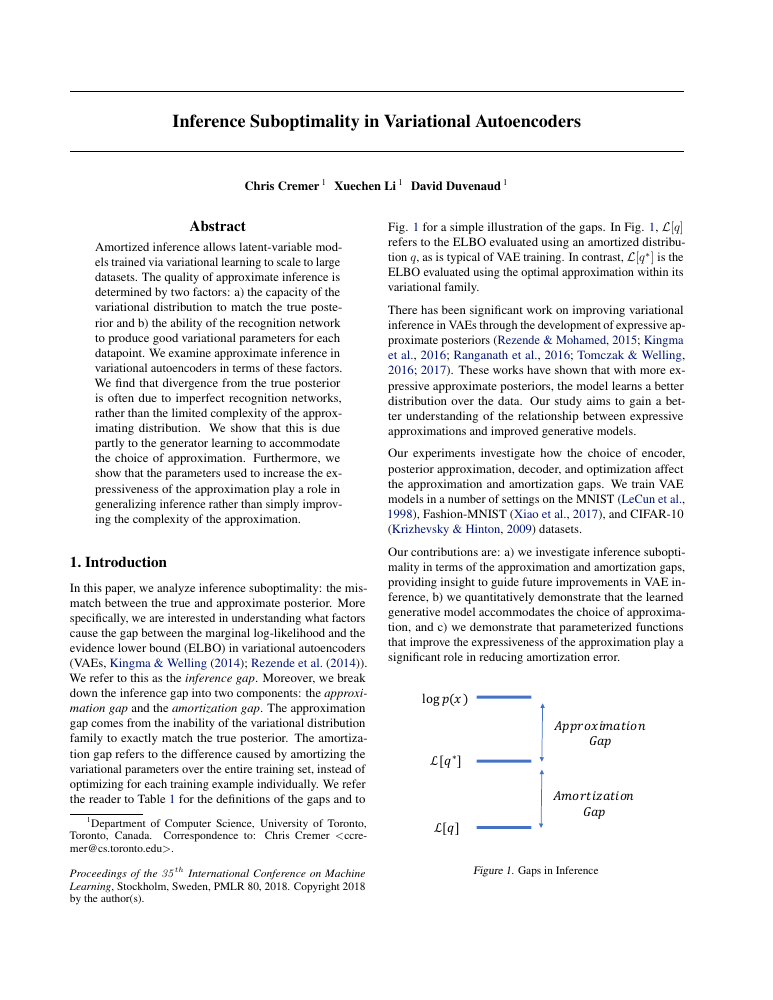
Inference Suboptimality in Variational Autoencoders
The move. Split inference error into the family's limitation and the inference network's shortfall within that family.
Read with AEVB · Normalizing flows · Semi-amortized VI · When amortization works
The idea and the mathematics
A poor encoder-based posterior fit can have two different causes: the family may be too restrictive, or the encoder may fail to find a good member of that family. These call for different remedies.
This paper analyzes inference in VAEs by separating the best fit available within a family from the fit produced by an encoder. For a fixed generative model, these become approximation and amortization gaps. Experiments also examine how the learned model adapts to its inference procedure. Its contribution is a diagnosis of distinct errors, rather than a new bound or posterior family.
For each observation, let \(q_x^\star\) be the best member of the chosen local family and \(q_\phi(\cdot\mid x)\) the encoder output. Insert and subtract \(\mathcal L[q_x^\star]\):
The first measures what the family can represent. The second measures how well the encoder finds the best member for this observation. A richer family, as in Normalizing flows, can reduce the first. Improving the encoder or refining its output, as in Semi-amortized VI, can reduce the second.
Ask two different questions about a disappointing fit. Could this family represent a much better approximation? And did the encoder find that approximation? Imagine a curved posterior and a diagonal Gaussian encoder output. Moving and resizing the Gaussian separately for this observation may improve it substantially, but no such adjustment can make its contours follow the curve. The first improvement diagnoses amortization error; the remaining mismatch suggests a limitation of the family.
The paper operationalizes this distinction by fixing a trained generative model, locally optimizing variational parameters for individual observations, and comparing with the encoder's output. It also uses more expressive approximations and evidence estimates to investigate the residual gap. Its experiments show that amortization can account for a substantial part of inference suboptimality, so simply adding a richer family is not the only remedy.
How to use the diagnosis. If local refinement gives a large ELBO increase, improving the encoder, its inputs, or its refinement procedure is promising. If it gives little improvement but the fit remains inadequate, more expressive distributions deserve attention.
The ideal decomposition uses the best member of the family. In practice, a local optimizer may not find it, so an observed refinement gain measures a recoverable portion of the gap. Also, comparisons should hold the generative model fixed: retraining that model can reshape the posterior and change both gaps at once.
Semi-Amortized Variational Autoencoders
The move. Refine the encoder's local parameters with optimization steps and train through those steps.
Read with AEVB · Amortization gap · When amortization works
The idea and the mathematics
An encoder is fast because it shares inference work across observations, but its output may fall short of the best local fit. A few observation-specific optimization steps can refine that initial guess.
Semi-amortized VAEs use an encoder to initialize local variational parameters, refine them with ELBO optimization, and differentiate through that refinement during joint training. The local family and ELBO can stay unchanged. What changes is how local parameters are produced and how the encoder learns; this differs from fitting an encoder once and adding unrelated optimization only at test time.
An encoder gives a fast initial guess. Instead of accepting it as the final local fit, refine it:
Here \(\phi\) denotes the shared encoder parameters and \(\varphi^{(t)}\) the local variational parameters for one observation. Both parameterize the approximation; neither is a model parameter.
Train the encoder by differentiating the final objective through these refinement steps. It learns an initialization that works well after correction. More steps spend additional computation on the local problem.
Inference suboptimality identifies the amortization gap. This paper gives a way to reduce it while retaining a shared inference network.
Learn a starting point that is easy to repair. A standard encoder is trained to make its first answer good. A semi-amortized encoder is trained to make the answer after a small amount of inference good. These can be different starting points: an initialization slightly farther from the optimum may lie in a region where a few gradient steps are much more effective.
For one refinement step with fixed step size,
The Hessian term records how the correction changes when the initialization changes. Training through the refinement therefore teaches the encoder about the local optimization landscape. Merely refining at test time can improve a fit, but does not provide this training signal to the encoder.
The paper combines fast shared inference with local optimization and studies settings where ordinary amortized training underuses latent variables. More accurate local inference can make it harder for the generative model to avoid learning useful latent explanations.
The price is iterative inference. Each refinement adds evaluations, and differentiating through the sequence needs Hessian–vector products and additional memory or recomputation. Step sizes and optimization stability still matter; finite noisy steps need not all improve the ELBO. Refinement also remains within the selected variational family, so it targets amortization error without removing that family's approximation gap.
Amortized Variational Inference: When and Why?
The move. Ask whether the information given to an inference network is sufficient to express the optimal local fit.
Read with SVI · Amortization gap · Semi-amortized VI
The idea and the mathematics
An encoder can only use the information supplied to it. Before making the network larger, it is useful to ask whether those inputs are sufficient to determine the local variational fit we want it to predict.
This analysis compares separately optimized mean-field local factors with a shared inference function in latent-variable models. It asks when the model's dependence structure permits the encoder's inputs to determine an optimal local fit, and when those inputs must be expanded. It studies whether amortization can match factorized VI—not whether mean field can represent the exact posterior, or whether a trained finite network necessarily reaches the optimum.
For shared inference to attain the same optimum as freely chosen local factors, the optimal local parameters must be expressible as a function of the information supplied to the inference network. If the network sees only \(x_i\) and optimal local parameters require information from other observations, increasing network capacity alone leaves that issue unresolved. The paper characterizes when the gap can close and studies what happens when the inference function is allowed additional inputs. Amortization gap diagnoses the gap after fitting. When amortization works asks when the model structure makes the gap avoidable in principle.
Some missing information cannot be supplied by a larger network. Consider a hidden-state sequence. The same observed value \(x_i\) can appear in two positions, but neighboring observations may support very different states at those positions. A deterministic encoder seeing only \(x_i\) must return the same parameters both times. If the optimal local factors differ, no increase in its width or depth can make that restricted input sufficient.
The paper returns to the CAVI equation,
and asks which observations can affect its right-hand side. This connects the existence of an ideal inference function to the graphical structure of the model. In a simple hierarchical model, shared global information can be absorbed into the fitted mapping, leaving a suitable local dependence on \(x_i\). Other graphs require additional context; the paper analyzes examples with neighboring observations and denser dependencies.
The design lesson. Before enlarging an encoder, check whether it receives the information needed to distinguish the local inference problems. Sequence context, dataset summaries, or other model-appropriate inputs may matter more than capacity. Existence of an ideal function does not guarantee that training finds it, and a fitted mapping for one dataset need not automatically generalize when its global context changes. The structural question comes before the optimization question.
What can we prove about the fit?
Separate statistical accuracy, uncertainty estimates, gradient variance, and optimization convergence. They answer different questions about the same approximation.
First article page; publisher cover sheet omitted.
Frequentist Consistency of Variational Bayes
The move. Study concentration of the variational posterior as data grow, separately from optimization error.
Read with MFVI · Linear-response covariance · BBVI convergence
The idea and the mathematics
Successful optimization on one dataset does not tell us what happens as more data arrive. A separate statistical question is whether the optimized variational distribution concentrates around the data-generating parameter.
This paper studies the statistical behavior of variational Bayes as the dataset grows. Under its identifiability, testing, and local asymptotic assumptions, it establishes consistency and a variational Bernstein–von Mises result, connecting the limiting approximation to a KL projection. The contribution concerns the optimized variational solution; it does not provide a new gradient algorithm or guarantee that a numerical optimizer finds that solution.
The global unknown is a block \(z_g\) of \(z\); the question is what happens to its variational posterior as the dataset grows.
Profile out the local variational factors to obtain a variational criterion for the global parameter. Under regularity and local asymptotic normality conditions on this criterion, the appropriately rescaled VB posterior approaches the KL projection of a limiting Gaussian onto the variational family. There are two distinct claims: the unscaled approximation can concentrate at the true parameter, while its local, rescaled covariance can still differ from the limiting Gaussian’s covariance. This is a statistical result as the amount of data grows. Optimization guarantees instead ask how closely an algorithm can approach the variational optimum for a given dataset.
Getting the center right is different from getting uncertainty right. Suppose a two-dimensional posterior becomes approximately Gaussian with covariance
Its reverse-KL projection onto diagonal Gaussians has the same mean, but each variance is \((1-\rho^2)/N\). Both the true posterior and the projection concentrate as \(N\) grows. Yet their ratio of variances remains \(1-\rho^2\), so more data does not remove the relative underestimation of uncertainty. This is the local Gaussian version of the mean-field geometry.
The paper establishes a variational Bernstein–von Mises theory under assumptions on the profiled variational criterion. After centering and rescaling, the variational posterior behaves like a KL projection of a limiting normal distribution. This gives a route to consistency and asymptotic descriptions, rather than assuming that the computational approximation becomes exact with enough data.
What the theorem depends on. The variational criterion must have the appropriate local asymptotic behavior and concentrate around the relevant parameter. Poor identification, an inconsistent profiled criterion, or other failures of these conditions can invalidate the conclusion. The theory concerns the variational solution itself; an algorithm trapped at a poor local solution is a separate issue. For uncertainty correction at a fitted solution, linear response takes a different route.
Covariances, Robustness, and Variational Bayes
The move. Estimate covariance from how reoptimized variational means respond to a small target perturbation.
Read with MFVI · Amortization gap · VB consistency
The idea and the mathematics
Mean field can estimate posterior means well while giving poor variances and no cross-covariances. How those fitted means respond to a small change in the target offers another route to measuring uncertainty.
Linear-response VI starts from a fitted variational optimum and studies how its means respond to a small perturbation of the target. This yields covariance estimates and local robustness measures even when mean field itself has no cross-covariances. The fitted family is not made more expressive: the improvement is in the uncertainty calculation, relying on stable optimization and sufficiently accurate nearby variational means.
Let \(\delta\) be a small perturbation vector. Perturb the log posterior by \(\delta^\top g(z)\). For the exact perturbed posterior, differentiation gives
The paper substitutes the response of reoptimized variational means for this derivative. If \(\phi^\star(\delta)\) solves \(\nabla_\phi\mathcal L_\delta=0\), implicit differentiation computes the response through the Hessian of \(\mathcal L\). The resulting covariance estimate can contain off-diagonal terms even when \(q\) factorizes. It measures how all fitted means move in response to a perturbation, which is a different calculation from taking covariance under the fitted \(q\) directly.
A small push reveals dependence. If increasing preference for larger \(z_1\) also moves the fitted mean of \(z_2\), the model contains a relationship between them, even if the fitted mean-field density has zero covariance. Reoptimizing after the push lets all factors respond together; simply drawing from the original factorized fit cannot reveal that response.
For a Gaussian target \(\mathcal N(m,\Sigma)\), the perturbation \(\delta^\top z\) changes its mean to \(m+\Sigma\delta\). A mean-field Gaussian fit recovers that mean for every nearby perturbation. Differentiating the fitted mean therefore recovers the full \(\Sigma\), including correlations absent from the factorized density. This example shows exactly what the correction measures.
Let \(a(\phi)=\mathbb E_{q_\phi}[g(z)]\) and \(H=\nabla_\phi^2\mathcal L(\phi^\star)\). At a smooth, isolated optimum, implicit differentiation gives the response estimate
In practice this can be computed through linear solves rather than forming an inverse. The same perturbation idea also measures local sensitivity to prior or model choices.
When to be cautious about the result. Accurate variational means at one point are not enough; their responses to nearby perturbations must be accurate too. A nearly singular Hessian, a change between competing optima, or a poor mean fit can make the correction unreliable. It improves a covariance estimate without turning the fitted \(q\) into a new distribution with those correlations.
Provable Gradient Variance Guarantees for Black-Box Variational Inference
The move. Bound location-scale gradient noise using target smoothness, noise moments, and the current parameters.
Read with AEVB · BBVI convergence · Mean-field convergence
The idea and the mathematics
To understand a stochastic optimizer, we need to understand the noise in its gradients. In VI, that noise changes with the location and spread of the approximation, so a single constant variance assumption can hide important behavior.
For location-scale approximations and a smooth negative log target, this paper bounds the size of reparameterization-gradient fluctuations using parameters, dimension, and base-noise moments. These are guarantees about an existing estimator. They retain the model and VI objective and expose why a uniform, parameter-independent noise bound can be the wrong assumption for convergence analysis.
For a location-scale sample \(z=m+B\epsilon\), the sampled gradient of a smooth function \(f(z)\) with respect to \(B\) is \(\nabla_z f(z)\epsilon^\top\). Its squared norm contains both \(\|\nabla_z f(z)\|^2\) and \(\|\epsilon\|^2\). If \(f\) has a gradient that changes no faster than \(\beta\) times the change in its input (called \(\beta\)-smoothness), and \(\bar z\) is a stationary point, then \(\|\nabla_z f(z)\|\leq \beta\|z-\bar z\|\). Combining this with standardized base-noise moments bounds the gradient second moment in terms of \((d+1)\|m-\bar z\|^2\) and \((d+\kappa)\|B\|_F^2\), scaled by \(\beta^2\), with \(\kappa\) the base fourth moment in the paper’s setup. The new contribution is a quantitative gradient-noise bound. BBVI convergence turns bounds of this type into optimization results.
Why the scale gradient can be noisier than the mean gradient. Moving \(m\) shifts every draw equally, so its sampled derivative is \(\nabla_z f(z)\). Changing \(B\) changes the direction and size of each noise realization, producing the outer product \(\nabla_z f(z)\epsilon^\top\). Large noise affects both the location at which the function is evaluated and the multiplier in its gradient.
For the scalar quadratic \(f(z)=\tfrac12 z^2\), take \(m=0\), \(z=s\epsilon\), and standard Gaussian noise. The scale-gradient estimate is \(s\epsilon^2\), giving
The noise grows with the scale being optimized. A global assumption that gradient variance is bounded by one fixed constant would conceal this dependence. The paper instead relates second moments to the location and spread of the approximation, with explicit dimension and base-noise moment factors.
What the bound tells us. Smoothness limits how quickly the function's gradient can grow away from a stationary point; the base fourth moment controls how often noise produces large products. Heavy tails or an unbounded Hessian can break this particular argument. The result supports optimization theory rather than proving that every practical model has low variance. Convergence analysis uses this parameter-dependent view of noise.
Provable convergence guarantees for black-box variational inference
The move. Use iterate-dependent variance bounds to analyze projected and proximal VI algorithms.
Read with Gradient variance bounds · STL convergence · Mean-field convergence
The idea and the mathematics
A usable gradient estimator does not by itself prove that optimization converges. Gaussian VI has two features a convergence argument must handle: parameter-dependent gradient noise and an entropy term that becomes steep near a collapsing covariance.
With dense Gaussian approximations parameterized by a mean and scale matrix, this paper uses quadratic noise bounds to analyze projected and proximal stochastic-gradient VI. Smoothness and convexity assumptions on the negative log target govern the guarantees. Its contribution connects an existing ELBO estimator to provably convergent optimization; it does not claim convergence for arbitrary neural-network parameterizations or multimodal targets.
Write the negative ELBO as a sum
where \(f\) is the expected negative log target and \(h=-\mathcal H(q_\phi)\) is the negative entropy. Estimate the gradient of the first part with \(\widehat g_\phi\). A proximal update then chooses a nearby parameter value by solving a small optimization problem that includes the entropy term exactly:
The proximal step balances a gradient proposal against the entropy term instead of treating both as noisy derivatives.
The paper's Gaussian-family analysis allows gradient noise to depend on the current parameters through a quadratic bound. Combined with smoothness and convexity assumptions, this gives convergence guarantees for projected and proximal algorithms.
Gradient variance bounds asks how noisy one update is. This paper asks how those updates accumulate into progress. STL convergence sharpens the picture when noise vanishes near the optimum.
Entropy creates a barrier against collapse. For one Gaussian scale \(s\gt 0\), the negative entropy contains \(-\log s\). Its derivative becomes arbitrarily steep near zero, so a generic smooth-objective analysis is awkward. The proximal step handles this term as a small exact optimization problem.
If a gradient step on the expected negative log target proposes a scale \(v\), the entropy correction solves
The result is positive even if the unconstrained proposal \(v\) was negative. This simple calculation explains why separating the tractable entropy from the sampled target term is useful: the algorithm can respect scale geometry directly.
The paper combines such optimization structure with bounds on how stochastic gradient noise grows as the approximation moves. For suitable Gaussian parameterizations and target assumptions, this yields convergence rates instead of relying on a uniformly bounded-noise assumption.
The distinction from CAVI. A proximal stochastic step is not the exact maximization of one factor and need not improve the ELBO on every realization. The guarantees describe accumulated progress under their assumptions. Strongly nonconvex targets, nonlinear reparameterizations that destroy the required geometry, or heavy-tailed noise can fall outside those guarantees. The result explains a principled optimizer for a defined setting, rather than guaranteeing success for every black-box model.
Black Box Variational Inference with a Deterministic Objective: Faster, More Accurate, and Even More Black Box
The move. Reuse a fixed set of noise draws to turn the sampled objective into a deterministic optimization problem.
Read with ADVI · Learned quadratic controls · BBVI convergence
The idea and the mathematics
With fresh Monte Carlo draws at every evaluation, the estimated ELBO changes even when the parameters do not. Holding the underlying noise fixed turns those repeated evaluations into comparisons on one stable surface.
DADVI fixes the base-noise draws and optimizes their sample-average approximation to the mean-field Gaussian VI objective. This replaces resampling at every iteration with a single deterministic surface, enabling second-order optimization, error assessment, and linear response. The population target remains the ELBO, but the finite-sample objective is an approximation to it, not merely an unbiased gradient evaluated repeatedly.
Write \(\ell_\phi(\epsilon)=\log\gamma(T_\phi(\epsilon))-\log q_\phi(T_\phi(\epsilon))\) for a sampled ELBO contribution.
Draw \(\epsilon^{(1)},\dots,\epsilon^{(K)}\) once and optimize
using the same draws at every iteration. The evaluated function is now deterministic conditional on those draws, so standard second-order optimization becomes practical. There is still Monte Carlo error: the maximizer of \(\widehat{\mathcal L}_K\) is a random approximation to the maximizer of \(\mathcal L\). This differs from Learned quadratic controls, which improves the stochastic gradient of the original objective. DADVI optimizes a fixed random approximation to that objective.
Fixing the draws makes comparisons repeatable. With fresh randomness at every evaluation, a line search can see a better value simply because it received luckier samples. DADVI holds the base noise fixed, so every candidate parameter setting is judged using the same random reference points. The samples in latent space still move with the parameters: \(z^{(s)}=T_\phi(\epsilon^{(s)})\). It is the noise that is frozen, not the resulting \(z^{(s)}\).
For a scalar Gaussian target, using exact entropy and fixed Gaussian draws gives, up to constants,
Writing \(\bar\epsilon\) for their mean and \(v_\epsilon\) for their empirical variance with denominator \(K\), the optimizer is \(s=1/\sqrt{v_\epsilon}\), \(m=-s\bar\epsilon\). Even perfect numerical optimization therefore retains error from this particular set of draws. Fresh draws can be used to assess that error separately from optimization convergence.
Why the family matters. The paper analyzes favorable mean-field behavior, but also shows a failure for unrestricted full-rank fitting when there are too few fixed draws relative to dimension. Directions unobserved by the draws can allow covariance expansion without the sampled target term detecting it. Deterministic optimization is powerful because it exposes a stable objective; that objective must still be a sufficiently informative approximation to the true expectation.
Linear Convergence of Black-Box Variational Inference: Should We Stick the Landing?
The move. Connect vanishing gradient noise near an exact fit to geometric convergence of the optimizer.
Read with Sticking the Landing · Gradient variance bounds · BBVI convergence
The idea and the mathematics
Persistent gradient noise can keep pushing an optimizer around near a solution. Sticking the Landing offers a different possibility: when the approximation matches the target, its sampled gradient vanishes for every draw.
This paper analyzes STL gradient noise and projected BBVI for location-scale families under smoothness and log-concavity conditions. When the family can represent the target exactly, vanishing noise yields geometric convergence in the stated setting; misspecification introduces a residual term. The advance is a convergence guarantee tied to estimator and family properties, rather than a new ELBO or a claim that STL always outperforms every alternative.
Sticking the Landing shows pointwise cancellation at an exact fit. This paper proves a bound that controls STL gradient noise as the parameters approach the solution. Under perfect variational-family specification and the paper’s smoothness and convexity conditions, the variance bound vanishes quadratically with distance to the optimum, allowing geometric convergence. Under misspecification, a residual term can remain. The new result is the link between an estimator’s variance near the solution and the optimizer’s convergence rate.
An optimizer behaves differently when its noise disappears at the solution. With persistent gradient noise, a fixed step size tends to keep pushing the parameters around even after they approach the optimum. Decreasing the step size suppresses those pushes but also slows progress. If the noise shrinks with the remaining error, the algorithm can keep taking effective steps without the same noise floor.
A schematic form of the paper's bound is
where the residual term reflects mismatch between the variational family and target. Under perfect specification, STL's cancellation removes this residual. Together with the required strong convexity and smoothness, this supports geometric contraction of the optimization error.
A correlated Gaussian explains the limitation. A full-rank Gaussian family can match a Gaussian posterior exactly. A diagonal family cannot match a strongly correlated Gaussian, so spatial log-density gradients still disagree at its best fit. STL then retains a random component. The paper quantifies misspecification through a score-discrepancy quantity and shows settings where STL can be worse than an estimator using closed-form entropy.
Thus this result gives a reason to expect particularly fast optimization when the family is well matched, not an unconditional preference for STL. The estimator, the family, and the parameterization jointly determine whether the noise vanishes where the optimizer is trying to go.
Nearly Dimension-Independent Convergence of Mean-Field Black-Box Variational Inference
The move. Exploit diagonal scale structure to sharpen the explicit dimension dependence of iteration bounds.
Read with MFVI · Gradient variance bounds · BBVI convergence
The idea and the mathematics
A full covariance approximation has many more scale parameters than a mean-field approximation. This difference also changes which random products appear in their gradients, suggesting that their optimization bounds should reflect that structure.
This result specializes to mean-field location-scale approximations and strongly log-concave, log-smooth targets. Diagonal scale structure sharpens the explicit dimension dependence of BBVI iteration bounds to logarithmic for sub-Gaussian families. It analyzes optimization within that family. It neither removes the approximation error caused by independence nor makes the cost of processing a \(d\)-dimensional gradient independent of \(d\).
Restrict the location-scale family to mean field, so the scale matrix is diagonal. The gradient with respect to its scales then has components \(\partial_{z_i}f(z)\epsilon_i\) rather than all products \(\partial_{z_i}f(z)\epsilon_j\). The proof exploits this structure to sharpen the variance bound. For strongly log-concave, log-smooth targets and a sub-Gaussian family, the explicit dimension factor in the iteration bound is \(O(\log d)\), compared with \(O(d)\) for the full-rank bound discussed in the paper. This concerns iterations to optimize within the chosen family. The mean-field restriction can still increase the approximation gap, and the iteration count is distinct from the cost per iteration.
Count which random products the optimizer has to learn. A full scale matrix has entries \(B_{ij}\), and every such derivative contains the product \(\partial_{z_i}f\,\epsilon_j\). A diagonal scale needs only the matching-coordinate products \(\partial_{z_i}f\,\epsilon_i\). The paper shows that exploiting this structure in the analysis can give a much sharper noise bound than treating the diagonal case as an arbitrary full matrix with many zeros.
For sub-Gaussian noise, the largest coordinate fluctuations grow much more slowly with dimension than the sum of all squared fluctuations. Roughly, \(\mathbb E\max_i\epsilon_i^2\) grows like \(\log d\), while \(\mathbb E\|\epsilon\|^2\) grows like \(d\). This offers intuition for the improved explicit dimension factor in the proof. The paper also derives weaker dimension dependence for heavy-tailed families with finitely many moments, and a sharper result when the target Hessian is constant.
What nearly dimension-independent does not mean. Evaluating a \(d\)-dimensional target and updating its parameters still costs computation. Other quantities in the rate, such as conditioning and initial error, can also depend on the problem dimension. Most importantly, rapid convergence to the best mean-field approximation says nothing by itself about its posterior accuracy. A highly correlated target can be easy to optimize within that restricted family and still be poorly represented. Read this alongside mean-field geometry, not as a reason to ignore it.